Reading notes of major advances in NLP Transfer learning published in 2018:
- ELMo from Allen NLP: Deep Contextualized Word Representations
- ULMFiT from fast.ai: Universal Language Model Fine-tuning for Text Classification
- Transformer from OpenAI: Improving Language Understanding by Generative Pre-Training
- BERT from Google: BERT: Pre-training of Deep Bidirectional Transformers for Language Understanding
Feature-Based Approaches
Word Embedding
Pre-trained word embeddings is the most widely-adopted transfer learning method in NLP. Since the introduction of word2vec in 2013, the standard way of doing NLP projects is to use pre-trained word embeddings to initialize the first layer of a neural network, the rest of which is then trained on data of a particular task.
As it evolves from word2vec to GloVe to sub-word embeddings fasText, word embeddings have been immensely influential. However, they have their limitations, such as
- they only incorporate previous knowledge in the first layer of the model while the rest of the network needs to be trained from scratch.
- they only have a single context independent representation for each word and can’t address polysemy.
ELMo: Contextualized Embeddings from Language Models
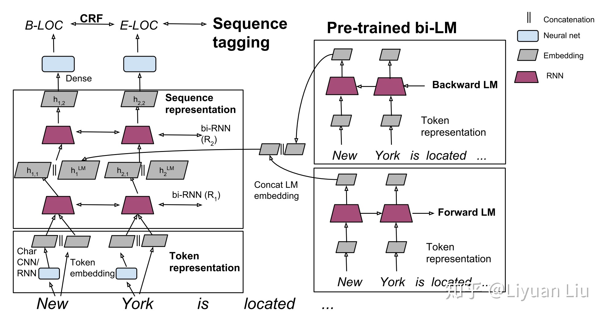
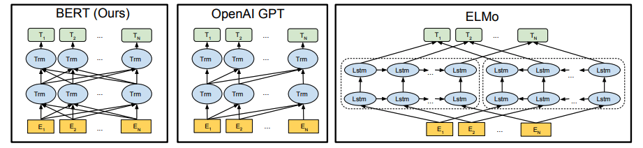
ELMo address the polysemy limitation by introducing a deep contexualized word representation (ElMo) that improves the state of the art across a range of language understanding problems. ELMo word representations are functions of the entire input sentence, computed on top of two-layer biLMs.
The state-of-the-art bidirectional neural language models compute a token representation $\textbf{x}{k}^{LM}$ then pass it through $L$ layers of forward LSTMs. At each position $k$, the $j$-th LSTM layer outputs a context-dependent representations $\textbf{h}{k,j}^{LM}$, where each representation is a concatenation of the forward and backward representation$[ \overrightarrow{\textbf{h}}{k,j}^{LM}, \overleftarrow{\textbf{h}}{k,j}^{LM}]$.
ELMo is a task specific combination of the intermediate layer representations in the biLM. For each token $t_k$, a $L$-layer biLM computes a set of $2L + 1$, where $\textbf{h}_{k,0}^{LM}$ is the token layer representation $x_k^{LM}$. For inclusion in a downstream model, ELMo collapses all layers into a single vector with task specific weighting:
\[\textbf{ELMo}_k^{task} = \gamma^{task} \sum_{j=0}^L s^{task}_j \textbf{h}_{k,j}^{LM}\]Most supervised NLP models form a context-independent token representations $\textbf{x}k$ for each token position using pre-trained word embedding and optionally character-based representations. Then the model forms a context-sensitive representations $\textbf{h}{k}$ with RNNs, CNNs or feed forward networks.
To add ELMo to the supervised model, the authors
- Freeze the weights of the biLM, run the biLM and record all of the layer presentations for each word
- Replace $\textbf{x}_k$ with $\left[\textbf{x}_k; \textbf{ELMo}_k^{task}\right]$ and pass them into the task RNN
- Let the end task model learn a linear combination of these representations
For some tasks, the authors observe further improvement by introducing another set of output specific linear weights and replacing $\textbf{h}_k$ with $\left[\textbf{h}_k; \textbf{ELMo}_k^{task}\right]$. The authors also found it beneficial to add a moderate amount of dropout to ELMo and in some cases to regularize the ELMo weights by adding L2 loss, which forces the ELMo weights to stay close to an average of all biLM layers.
Fine-tuning Approaches
Universal Language Model Fine-tuning (ULMFiT)
Instead of using a pre-trained Language Model as contextualized word embedding, Howard and Ruder proposed ULMFiT, a method to fine-tune Language Models pre-trained on a large general-domain corpus to any downstream target task.
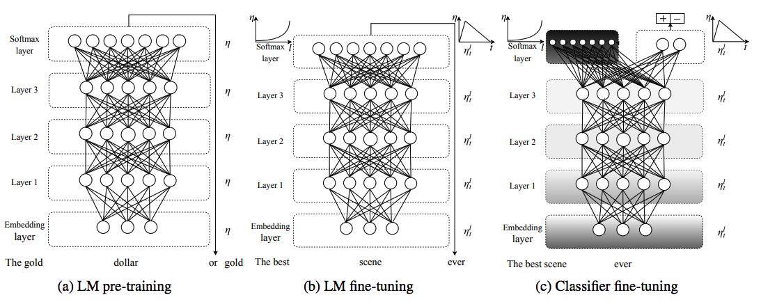
As shown in the figure above, ULMFit consists of three stages of training
- General-domain LM pretraining: A LM is trained on a large general-domain corpus to capture general properties of language. While this stage is the most expensive, it only needs to be performed once and there are many pre-trained LM available for download.
- Target task LM fine-tuning: The data of the target task will likely come from a different distribution. Thus we fine-tune the LM on data of the target task without the label.
- Target task classifier fine-tuning: The LM is augmented by 2 linear blocks to form a classifier, which is then fine-tuned on the labeled target task dataset.
The paper also introduced quite a few fine-tuning tricks that the authors empirically found it to work well.
- Discriminative fine-tuning: tune each layer with different learning rate.
- Slanted triangular learning rates: a learning rate schedule similar to the cyclic learning rates, but with a short increase and a long decay period
- Gradual unfreezing: gradually unfreeze the model starting from the last layer. First unfreeze the layer layer and fine-tune all un-frozen layers for one epoch. Then unfreeze the next lower and repeat till we fine-tune all layers until convergence.
OpenAI GPT: adding Transformers to LM
Five months after ULMFiT, OpenAI provided an incremental improvement on the fine-tuning concept by upgrading the previous state-of-the-art AWD-LSTM Language model to a Transformer-based LM. The LM is a multi-layer Transformer decoder, which applies a multi-headed self-attention operation over the input context tokens followed by position-wise feedforward layers to produce an output.
\(h_0 = UW_e + W_p\) \(h_l = \text{transformer_block}(h_{l-1}) \forall i \in [1, n]\) \(P(u) = \text{softmax}(h_{n}W_e^T)\)
where $U = (u_{-k}, \cdots, u_{-1})$ is the context vector of tokens, $W_e$ is the token embedding matrix and $W_p$ is the position embedding matrix.
To fine-tune the LM for a supervised task, an linear block is added to the above LM. The final transformer block’s activation $h_l^m$ is connected into an added linear output layer with parameters $W_y$ to predict $y$.
\[P(y|X) = \text{softmax}(h_{l}^mW_y)\]The authors also found that including language modeling as an auxiliary object to the fine-tuning helped learning by improving generalization of the supervised model and accelerating convergence. The overall objective is $L_{total} = L_{supervised} + \lambda \cdot L_{LM}$
Fine-Tuning
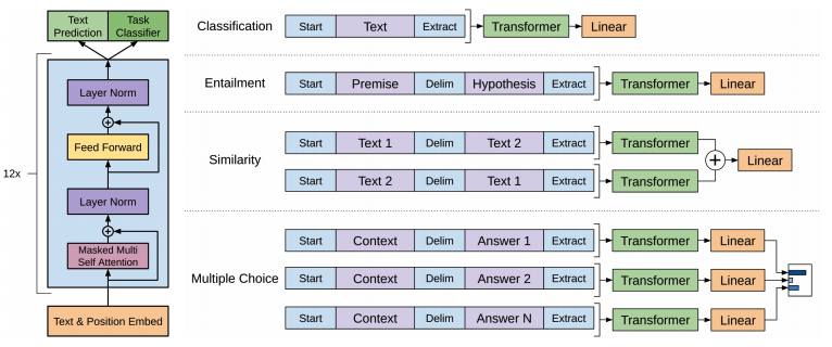
Some tasks like question answering or textual entailment requires structured inputs. The authors used a traversal-style where structured inputs are converted into a ordered sequence that directly fit into the pre-trained LM. These input transformations allow us to avoid making extensive changes to the architecture across tasks.
BERT: Let’s make it bidirectional
A major limitation in OpenAI GPT is that the transformer decoder architecture are unidirectional, where every token can only attend to previous tokens in the self-attention layers of the Transformer. This is sub-optimal for task that requires incorporating context from both directions. Devlin et al. from Google proposed Bidirectional Encoder Representations from Transformers (BERT) to address the unidirectional constraints.
Masked LM
Standard conditional language models can only be trained left-to-right or right-to-left since bidirectional conditioning would allow each word to indirectly “see itself” in a multi-layered context. Devlin et al. proposed masked LM, where some percentage (15%) of the input tokens are masked at random and the LM is trained to predict those masked tokens.
Next Sentence Prediction
In order to train a model that understands sentence relationships, the authors added a binary next sentence prediction task to the pre-training. It’s found that adding the task is very beneficial to both QA and NLI tasks.
Fine-Tuning
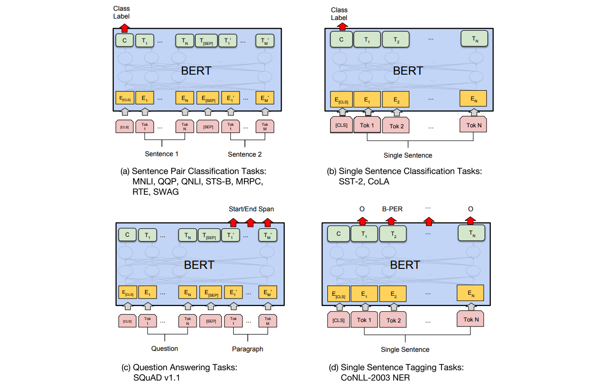
Same with the OpenAI GPT, BERT requires converting each task to be represented by a Transformer encoder architecture. A [CLS] token is added to the start of all input sentence. For sentence-level classification task, the final hidden state for the [CLS] token is connected into a linear layer and a softmax layer. For token-level task like NER, the final hidden state for each token $T_i$ is passed through a linear layer and a softmax layer for class probabilities.
Feature-based Approach
The feature-based approach like ELMo, where fixed features are extracted from the pre-trained model, has certain advantages. BERT can be used the exactly same way as ELMo, while not sacrificing much performance. On CoNLL-2003 NER, concatenating the token representations from the top four hidden layers of the pre-trained Transformer as an input to the LSTM, is only -0.3 F1 compared with fine-tuning the entire model. This approach is still +0.4 F1 compared with ELMo.