RNNs have been the state-of-the-art approach in modeling sequences. They align the symbol positions of the input and output sequences and generate a sequence of hidden states $h_t$ as a function of previous hidden state $h_{t-1}$ and the input for position $t$. This inherently sequential nature precludes parallelization .
In the paper Attention Is All You Need, Google researchers proposed the Transformer model architecture that eschews recurrence and instead relies entirely on an attention mechanism to draw global dependencies between input and output. While it achieves state-of-the-art performances on Machine Translation, its application is much broader.
P.S. the blog post by Jay Alammar has awesome illustration explaining the Transformer. the blog post on Harvard NLP also provides a working notebook type of explanation with some implementation.
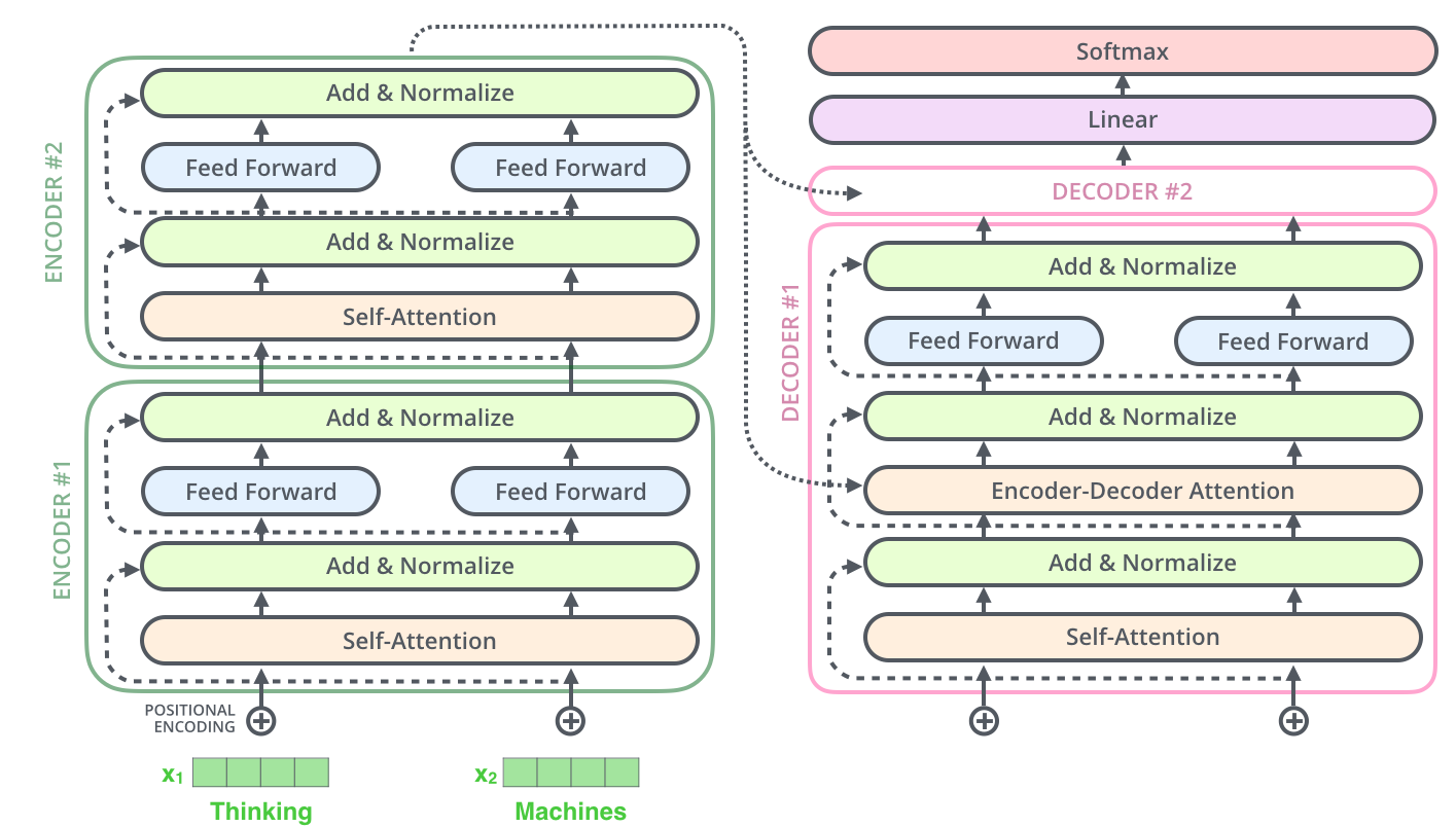
Model Architecture
 Model Architecture of Transformer (Credit)
The Transformer follows the Encoder-Decoder architecture. The encoder maps an input sequence $(x_1, \cdots, x_n)$ to a sequence of continuous representation $\textbf{z} = (z_1, \cdots, z_n)$. Given $\textbf{z}$, the decoder generates an output sequence $(y_1, \cdots, y_n)$ one step at a time. The model is auto-regressive, as the previous generated symbols are consumed as additional input at every step. The Transformer proposed several new mechanism that enabled abandoning recurrence, namely multi-head self-attention, point-wise feed-forward networks and positional encoding.
class EncoderDecoder(nn.Module):
    def __init__(self, encoder, decoder, input_embedding, output_embedding):
        super(EncoderDecoder, self).__init__()
        self.encoder = encoder
        self.decoder = decoder
        self.input_embedding = input_embedding
        self.output_embedding = output_embedding

    def forward(self, input_ids, output_ids):
        return self.decode(self.encode(input_ids), output_ids)

    def encode(self, input_ids):
        input_embedded = self.input_embedding(input_ids)
        return self.encoder(input_embedded)

    def decode(self, encoder_outputs, output_ids):
        output_embedded = self.output_embedding(output_embedded)
        return self.decoder(output_embedded, encoder_outputs)
1. Multi-Head Self-Attention
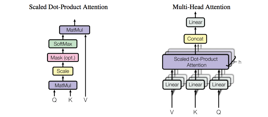 Scaled Dot-Product Attention and Multi-Head Attention (Credit)
Scaled Dot-Product Attention
Attention takes a query and a set of key-value pairs and output a weighted sum of the values. The Transformer uses the Scaled Dot-Product Attention, which takes the dot products of the query with all keys, divide each by $\sqrt{d_k}$ and apply a softmax function to obtain the weights on the value. Dividing the dot products by $\sqrt{d_k}$ prevents the its magnitude from getting too large and saturate the gradient on the softmax function.
\[\text{Attention}(Q,K,V) = \text{softmax} \left( \frac{QK^T}{\sqrt{d_k}}\right)V\]def scaled_dot_product_attention(Q, K, V, attn_mask):
# Q: [batch_size, n_heads, L_q, d_k]
# K: [batch_size, n_heads, L_k, d_k]
# V: [batch_size, n_heads, L_k, d_v]
d_k = Q.size(1)
unnormalized_attn_scores = torch.matmul(Q, K.transpose(-1, -2)) / np.sqrt(d_k) # scores : [batch_size, n_heads, L_q, L_k]
unnormalized_attn_scores.masked_fill_(attn_mask, -1e9) # Fills elements of self tensor with value where mask is one.
normalized_attn_scores = nn.Softmax(dim=-1)(unnormalized_attn_scores)
output = torch.matmul(normalized_attn_scores, V) # [batch_size, n_heads, L_q, L_v]
return output
Multi-Head Attention
The authors found it beneficial to linearly project the queries, keys and values $h$ times with different learned linear projections ($W_i^Q, W_i^K, W_i^V$). Attention is then performed in parallel on each of these projected versions. These are concatenated and once again projected by $W^O$ and result in the final values. Multi-head attention allows the model to jointly attend to information from different representation subspaces at different positions.
\(\text{MultiHead}(Q,K,V) = \text{Concat} \left( \text{head}_1, \text{head}_h\right)W^O\) \(\text{head}_i = \text{Attention}\left(QW_i^Q, KW_i^K, VW_i^V\right)\)
class MultiHeadAttention(nn.Module):
    def __init__(self, n_heads, hidden_size):
        super(MultiHeadAttention, self).__init__()
        self.hidden_size = hidden_size
        self.n_heads = n_heads
        self.d_model = int(self.hidden_size / self.n_heads)
        self.all_head_size = self.n_heads * self.d_model
        self.W_Q = nn.Linear(self.hidden_size, self.all_head_size)
        self.W_K = nn.Linear(self.hidden_size, self.all_head_size)
        self.W_V = nn.Linear(self.hidden_size, self.all_head_size)

    def forward(self, Q, K, V, attn_mask):
        # d_k = d_v = d_model
        # q: [batch_size, L_q, d_model]
        # k: [batch_size, L_k, d_model]
        # v: [batch_size, L_k, d_model]
        residual, batch_size = Q, Q.size(0)
        q_s = self.W_Q(Q).view(batch_size, -1, self.n_heads, self.d_model).transpose(1,2)  # [batch_size, n_heads, len_q, d_model]
        k_s = self.W_K(K).view(batch_size, -1, self.n_heads, self.d_model).transpose(1,2)  # [batch_size, n_heads, len_k, d_model]
        v_s = self.W_V(V).view(batch_size, -1, self.n_heads, self.d_model).transpose(1,2)  # [batch_size, n_heads, len_k, d_model]

        attn_mask = attn_mask.unsqueeze(1).repeat(1, self.n_heads, 1, 1) # attn_mask : [batch_size, n_heads, L_q, L_k]

        context = scaled_dot_product_attention(q_s, k_s, v_s, attn_mask)  # [batch_size, n_heads, len_q, d_model]
        context = context.transpose(1, 2).contiguous().view(batch_size, -1, self.all_head_size) # [batch_size, len_q, n_heads * d_model]
        output = nn.Linear(self.all_head_size, self.hidden_size)(context)
        return output
Three types of Attention Mechanisms
- In the attention layers between an Encoder and a Decoder, the queries come from the decoder and the key-value pairs come from the encoder. This allow every position in the decoder to attention over all the positions in the encoder.
- The attention layers in the Encoders serve as self-attentions, where each position in the later encoder and attend to all positions in the previous layer of encoder.
- The attention layers in the Decoders are also self-attention layers. In order to prevent leftward information flow and preserve the auto-regressive property (new output consumes previous outputs to the left, but not the other way around), all values in the input that correspond to illegal connection are masked out as $-\infty$.
2. Position-wise Feed-forward Networks
Each of the Feed-Forward (also called Fully-Connected) layers is applied to each position separately and identically. It consists of two linear transformations with a ReLU activation in between.
\[FFN(x) = \text{max}(0, xW_1 + b_1)W_2 + b_2\]class PositionwiseFeedForward(nn.Module):
def __init__(self, d_model, d_ff, dropout=0.1):
super(PositionwiseFeedForward, self).__init__()
self.w_1 = nn.Linear(d_model, d_ff)
self.w_2 = nn.Linear(d_ff, d_model)
self.dropout = nn.Dropout(dropout)
def forward(self, x):
return self.w_2(self.dropout(F.relu(self.w_1(x))))
3. Positional Encoding
In order for the model to make use of the order of the sequence, the paper introduces positional encoding, which encodes the relative or absolute position of the tokens in the sequence. The positional encoding is a vector that is added to each input embedding. They follow a specific pattern that helps the model determine the distance between different words in the sequence. For each dimension of the vector, the position of the token are encoded along with the sine/cosine functions.
\[\text{PE}_{(pos,2i)} = sin\left(\frac{pos}{10000^{2i/d_{model}}}\right) \ \ \ \ \ \ \text{PE}_{(pos,2i+1)} = cos\left(\frac{pos}{10000^{2i/d_{model}}}\right)\]The intuition is that each dimension corresponds to a sinusoid with wavelengths from $2\pi$ to $10000 \cdots 2\pi$ and it would allow the model to learn to attention by relative positions, since for any fixed offset $k$, $PE_{pos+k}$ can be represented as a linear function of $PE_{pos}$. As shown in the figure below, the earlier dimensions have smaller wavelengths and can capture short range offset, while the later dimensions can capture longer distance offset. While I understand the intuition, I am quite doubtful about whether this really work.
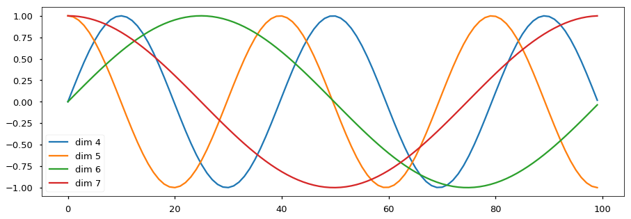 Examples of Sinusoid with different wavelengths for different dimensions (Credit)
class PositionalEncoding(nn.Module):
    def __init__(self, embedding_size, max_len=64):
        super(PositionalEncoding, self).__init__()

        # Compute the positional encodings once in log space.
        pe = torch.zeros(max_len, embedding_size)
        position = torch.arange(0, max_len).unsqueeze(1)
        div_term = torch.exp(torch.arange(0, embedding_size, 2) *
                             -(math.log(10000.0) / embedding_size))
        pe[:, 0::2] = torch.sin(position * div_term)
        pe[:, 1::2] = torch.cos(position * div_term)
        pe = pe.unsqueeze(0)
        self.register_buffer('pe', pe)

    def forward(self, x):
        return Variable(self.pe[:, :x.size(1)], requires_grad=False)
Discussion on Self-Attention
The authors devoted a whole section of the paper to compare various aspects of self-attention to recurrent and convolutional layers on three criteria:
- Complexity is the total amount of computation needed per layer.
- Sequential Operations is the minimum number of required sequential operations. These operations cannot be parallelized and thus largely determine the actual complexity of the layer.
- Maximum Path Length is the length of paths forward and backward signals have to traverse in the network. The shorter these path, the easier it is to learn long-range dependencies.
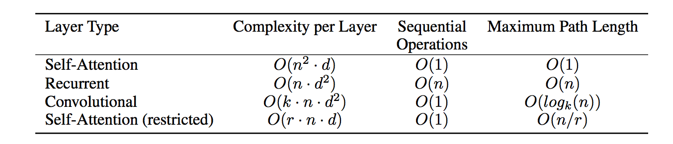 Complexity Comparison of Self Attention, Convolutional and Recurrent Layer. (Credit)
In the above table, $n$ is the sequence length, $d$ is the representation dimension, $k$ is the kernel size of convolution and $r$ is the size of the neighborhood in restricted self-attention.
Recurrent Layer
Computing each recurrent step takes $O(d^2)$ for matrix multiplication. Stepping through the entire sequences of length $n$ takes a total computation complexity of $O(nd^2)$. The Sequential Operations and Maximum Path Length are $O(n)$ due to the sequential nature.
Convolutional Layer
Assuming the output feature map is $n$ by $d$, each 1D convolution takes $O(k \cdot d)$ operation, making the total complexity $O(k \cdot n \cdot d^2)$. Since convolution is fully parallelizable, the Sequential Operations is $O(1)$. A single convolutional layer with kernel width $k < n$ does not connect all pairs of input and positions, thus requiring a stack of $O(n/k)$ contiguous kernels, or $O(log_k(n))$ in case of dilated convolutions.
Self-Attention Layer
Computing the dot product between the representations of two positions take $O(d)$. Computing the attention for all pairs of positions takes $O(n^2d)$. The compute is parallelizable, the Sequential Operations is $O(1)$. The self-attention layer connects all positions with a constant number of operations since there is a direct connection between any two positions in input and output. $O(1)$
Self-Attention Layer with Restriction
To improve the computational performance for tasks involving very long sequences, self-attention can be restricted to considering only a neighborhood size of $r$ centered around the respective position. This decreases the total complexity to $O(r\cdot n \cdot d)$, though it takes $O(n/r)$ operations to cover the maximum path length.
Training
- Training time: full model takes 3.5 days to train on 8 NVIDIA P100 GPUs. :0
- Optimizer: Adam. Increase learning rate for the first warmup_steps training steps and decrease it thereafter. Similar cyclic learning rate or the Slanted Triangular LR in ULMFiT
- Regularization:
- Residual dropout: apply dropout to output layer before the residual connection and layer normalization $P_{drop} = 0.1$
- Embedding dropout: apply dropout to the sums of the embeddings and the positional encodings $P_{drop} = 0.1$
- Label Smoothing of $\epsilon_{ls} =0.1$. This hurts perplexity but improves BLEU score.
PyTorch Implementation
class AddAndNorm(nn.Module):
    def __init__(self, hidden_size, dropout=0.1):
        super(AddAndNorm, self).__init__()
        self.dropout = nn.Dropout(dropout)
        self.norm = nn.LayerNorm(hidden_size)

    def forward(self, x, sublayer):
        return self.norm(x + self.dropout(sublayer(x)))


class Embedding(nn.Module):
    def __init__(self, embedding_size, vocab_size, max_len, use_positional_encoding=False):
        super(Embedding, self).__init__()
        self.use_positional_encoding = use_positional_encoding
        self.tok_embed = nn.Embedding(vocab_size, embedding_size)  # token embedding
        self.norm = nn.LayerNorm(embedding_size)
        if self.use_positional_encoding:
            self.pos_embed = PositionalEncoding(embedding_size, max_len)
        else:
            self.pos_embed = nn.Embedding(max_len, embedding_size)  # position embedding

    def forward(self, input_id):
        # (batch, seq)
        seq_len = input_id.size(1)
        pos = torch.arange(seq_len, dtype=torch.long)
        pos = pos.unsqueeze(0).expand_as(input_id)  # (seq_len,) -> (batch_size, seq_len)
        embedding = self.tok_embed(input_id) + self.pos_embed(pos)
        return self.norm(embedding)


class EncoderLayer(nn.Module):
    def __init__(self, n_heads, hidden_size, d_ff, dropout=0.1):
        super(EncoderLayer, self).__init__()
        self.self_attention = MultiHeadAttention(n_heads, hidden_size)
        self.ffn = PositionwiseFeedForward(hidden_size, d_ff)
        self.norm_1 = AddAndNorm(hidden_size)
        self.norm_2 = AddAndNorm(hidden_size)

    def forward(self, x, mask):
        att_output = self.norm_1(x, lambda x: self.self_attention(x, x, x, mask))
        ffn_output = self.norm_2(att_output, self.ffn)
        return ffn_output

class DecoderLayer(nn.Module):
    def __init__(self, n_heads, hidden_size, d_ff, dropout=0.1):
        super(DecoderLayer, self).__init__()
        self.self_attention = MultiHeadAttention(n_heads, hidden_size)
        self.encoder_decoder_attention = MultiHeadAttention(n_heads, hidden_size)
        self.ffn = PositionwiseFeedForward(hidden_size, d_ff)
        self.norm_1 = AddAndNorm(hidden_size)
        self.norm_2 = AddAndNorm(hidden_size)
        self.norm_3 = AddAndNorm(hidden_size)

    def forward(self, x, encoder_outputs, src_mask, target_mask):
        # x: output embedding
        # encoder_outputs: output of the last encoder
        seq_len = x.size(1)
        decoder_decoder_mask = self.subsequent_mask(seq_len) & target_mask
        self_att = self.norm_1(x, lambda x: self.self_attention(x, x, x, decoder_decoder_mask))
        encoder_decoder_att = self.norm_2(self_att, lambda x: self.encoder_decoder_attention(x, encoder_outputs, encoder_outputs, src_mask))
        ffn_output = self.norm_3(encoder_decoder_att, self.ffn)
        return ffn_output

    def subsequent_mask(self, size):
	    "Mask out subsequent positions."
	    attn_shape = (1, size, size)
	    subsequent_mask = np.triu(np.ones(attn_shape), k=1).astype('uint8')
	    return torch.from_numpy(subsequent_mask) == 1


class OutputClassifier(nn.Module):
    def __init__(self, hidden_size, vocab):
        super(OutputClassifier, self).__init__()
        self.dense = nn.Linear(hidden_size, vocab)

    def forward(self, x):
        return F.log_softmax(self.dense(x), dim=-1)


class Transformer(nn.Module):
    def __init__(self, n_layers, n_heads, hidden_size, d_ff, max_len, input_vocab_size, output_vocab_size, embedding_size, dropout=0.1):
        super(Transformer, self).__init__()
        self.input_embedding = Embedding(embedding_size, input_vocab_size, max_len, use_positional_encoding=False)
        self.output_embedding = Embedding(embedding_size, output_vocab_size, max_len, use_positional_encoding=False)
        self.encoder_stack = nn.ModuleList([copy.deepcopy(EncoderLayer(n_heads, hidden_size, d_ff)) for _ in range(n_layers)])
        self.decoder_stack = nn.ModuleList([copy.deepcopy(DecoderLayer(n_heads, hidden_size, d_ff)) for _ in range(n_layers)])
        self.output_classifier = OutputClassifier(hidden_size, output_vocab_size)

    def forward(self, input_ids, output_ids, input_mask):
        input_embedded = self.input_embedding(input_ids)
        encoder_outputs = input_embedded
        for encoder in self.encoder_stack:
            encoder_outputs = encoder(encoder_outputs, input_mask)
        output_embedded = self.output_embedding(output_ids)
        decoder_outputs = output_embedded
        for decoder in self.decoder_stack:
            decoder_outputs = decoder(decoder_outputs, encoder_outputs, input_mask)
        logits = self.output_classifier(decoder_outputs)
        return logits