Intro
Mixture of Experts (MoE) has become increasingly popular in the LLM community, and for good reason. These models effectively maintain the scaling laws originally established for dense models while keeping inference costs relatively manageable – a compelling advantage in our era of ever-growing language models. To better understand how MoE architectures actually work under the hood, I decided to extend Andrej Karpathy’s awesome nanoGPT repository to support MoE architecture. My implementation, called nanoMoE, is available on GitHub for anyone interested.
The modification turned out to be quite straightforward: I adapted the feed-forward network (FFN) component of the GPT-2 architecture to use the Mixture of Experts approach and ran a series of small-scale pre-training experiments to gain some hands-on insights about training MoE models. Through these experiments, I was able to verify some of the core claims from Google’s seminal 2021 paper Switch Transformers: Scaling to Trillion Parameter Models with Simple and Efficient Sparsity.
Understanding MoE Architecture
Before diving into implementation details, let’s clarify what MoE actually is. In a standard transformer model, each layer processes all tokens through the same parameters. In an MoE model, we replace certain components (typically the feed-forward networks) with a collection of “expert” networks. A routing mechanism then decides which expert(s) should process each token.
The beauty of this approach is that for each input token, we only activate a small subset of the total parameters, creating sparsity during both training and inference. This sparsity allows us to scale to much larger parameter counts without proportionally increasing computation costs.
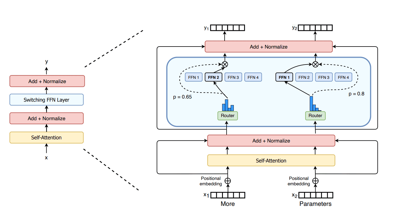
Figure 1: Illustration of a Mixture-of-Expert Layer from the Switch Transformer paper
The key components of the MoE Architecture include:
- Experts: Specialized neural networks (in our case, feed-forward networks) that each focus on different aspects of the input. For our implementation, we simply use the original FFN of GPT-2 for each expert.
- Router: A lightweight neural network that determines which expert(s) should process each token. In our implementation, this is a simple softmax layer.
- Gating Mechanism: Determines how to combine outputs when multiple experts process the same token (in some MoE variants). The gating mechanism in my implementation is top-k selection.
Implementing MoE in nanoGPT
NanoGPT provides a clean, minimalist implementation of the GPT-2 architecture, making it an ideal foundation for experimentation. Here’s how I extended it to support MoE:
class MoELayer(nn.Module):
    def __init__(self, config):
        super().__init__()
        self.ln_1 = LayerNorm(config.n_embd, bias=config.bias)
        self.attn = CausalSelfAttention(config)
        self.ln_2 = LayerNorm(config.n_embd, bias=config.bias)
        # normal transformers just have a MLP here
        # self.ffn = MLP(config)
        self.moe_ffn = MoEBlock(config)

    def forward(self, x):
        x = x + self.attn(self.ln_1(x))
        moe_output, routing_weights = self.moe_ffn(self.ln_2(x))
        x = x + moe_output
        return x, routing_weights


class MoEBlock(nn.Module):

    def __init__(self, config):
        super().__init__()
        self.n_embd = config.n_embd
        self.num_experts = config.num_experts
        self.top_k = config.top_k

        self.dropout = nn.Dropout(config.dropout)
        self.gate = nn.Linear(self.n_embd, self.num_experts, bias=False)
        self.experts = nn.ModuleList([MLP(config) for _ in range(self.num_experts)])

    def forward(self, x):
        batch_size, sequence_length, hidden_dim = x.shape
        # reshape x into 2-dimensional tensor for easier indexing across tokens
        x = x.view(-1, hidden_dim)  # (batch * seq, hidden_dim)
        router_logits = self.gate(x)  # (batch * seq, num_experts)
        routing_weights = F.softmax(router_logits, dim=-1, dtype=torch.float)
        routing_weights, selected_experts = torch.topk(routing_weights, self.top_k, dim=-1)
        # routing_weights (batch * seq, top_k)
        # selected_experts (batch * seq, top_k)
        # re-normalize the routing weights after top-k selection
        routing_weights /= routing_weights.sum(dim=-1, keepdim=True)
        # cast back to the input dtype
        routing_weights = routing_weights.to(x.dtype)

        # initialize an empty tensor to accumulate the output of each expert
        total_output_states = torch.zeros(
            (batch_size * sequence_length, hidden_dim), dtype=x.dtype, device=x.device
        )

        # One-hot encode the selected experts to create an expert mask
        # this will be used to easily index which expert is going to be solicited
        expert_mask = torch.nn.functional.one_hot(selected_experts, num_classes=self.num_experts).permute(2, 1, 0)
        # (batch * seq, top_k, num_experts) => (num_experts, top_k, batch * seq)
        # expert_mask[expert_idx][top_k_idx][token_idx] is 1 if the expert_idx-th expert is turned on
        # top_k_idx:  0 ... top_k
        # token_idx: token 0 ... batch_size * seq_length

        # Loop over all available experts in the model and perform the computation on each expert
        for expert_idx in range(self.num_experts):
            expert_layer = self.experts[expert_idx]
            top_k_idx, token_idx = torch.where(expert_mask[expert_idx])

            # current state: all token inputs related to this expert
            # Add None in order to broadcast
            current_state = x[None, token_idx].reshape(-1, hidden_dim)
            # forward the expert and then multiply by the weights
            current_hidden_states = expert_layer(current_state) * routing_weights[token_idx, top_k_idx, None]

            # Accumulate the expert output in the total_output_states buffer
            total_output_states.index_add_(0, token_idx, current_hidden_states.to(x.dtype))

        total_output_states = total_output_states.reshape(batch_size, sequence_length, hidden_dim)

        return total_output_states, router_logits
It’s worth noting that this implementation prioritizes clarity and readability over efficiency or scaling. The for-loop used in the forward function is intuitive for understanding the MoE mechanism but isn’t the most efficient approach on GPUs. More efficient and scalable implementations, such as the Block Sparse MoE layer introduced by MegaBlocks or the Expert Parallelism techniques mentioned in the Switch Transformer paper, are beyond the scope of this blog. Those optimizations would be necessary for production-scale implementations but would obscure the core concepts I wanted to highlight here.
Experimental Setup
To validate the MoE implementation and compare it with the standard GPT-2 architecture, I ran a series of experiments with the following configurations:
- Dense Model Baselines
- GPT-2 Small: Standard GPT-2 small (124M parameters)
- GPT-2 Medium: Standard GPT-2 medium (353M parameters)
- GPT-2 Large: Standard GPT-2 large (774M parameters)
- MoE Models
- GPT-2 Small 4e: GPT-2 small with 4 experts (293M parameters)
- GPT-2 Small 8e: GPT-2 small with 8 experts (520M parameters)
- GPT-2 Small 16e: GPT-2 small with 16 experts (973M parameters)
I’m running these experiments on fairly modest hardware – just 8x V100-32G GPUs. Without access to more substantial compute resources, I couldn’t run the GPT-2 XLarge variant or scale up my MoE experts further without implementing distributed training with Model Parallelization (which would significantly complicate the code).
For all experiments, I used consistent hyperparameters, keeping almost everything aligned with the original NanoGPT settings:
- Dataset: the OpenWebText corpus
- Total Batch size: ~0.5M tokens (adjusting local batch size and gradient accumulation steps across different models to maintain consistency)
- Learning rate: 6e-4 with cosine decay
- Training steps: 10,000
This means all models were pretrained on approximately 5B tokens. While this is relatively modest (about 1/60 of the training tokens that Andrej used for his GPT-2 small experiments), it’s sufficient to observe the patterns I’m interested in.
For context, here’s how this compares to the training compute used for modern LLMs:
| Model | Parameters | Training Tokens |
|---|---|---|
| GPT-2 Small (Mine) | 124M | 5B (val loss 3.15) |
| GPT-2 Small (Karpathy) | 124M | 300B (val loss 2.85) |
| LLaMA 1 | 7-65B | 1-1.4T |
| LLaMA 2 | 7-70B | 2T |
| LLaMA 3 | 8-405B | 16T |
| Qwen 2.5 | 0.5-70B | 18T |
Results
1. MoE models can be scaled up by adding more experts while keeping model FLOPS constant
This is the core advantage of MoE that seems almost too good to be true. With the same model FLOPS, the inference cost stays constant (achieving this takes tremendous engineering effort in practice) but the model performance continues to improve as we add more experts.
When you think about it, this makes perfect sense. Due to the sparse architecture, MoE effectively decouples the number of model parameters from the model FLOPS. As we add more experts, the model parameter count increases while computational requirements remain stable. So it’s no surprise that model performance improves, aligning perfectly with established scaling laws.
![]()
Figure 2: Performance scaling of Switch Transformer models with increasing expert count
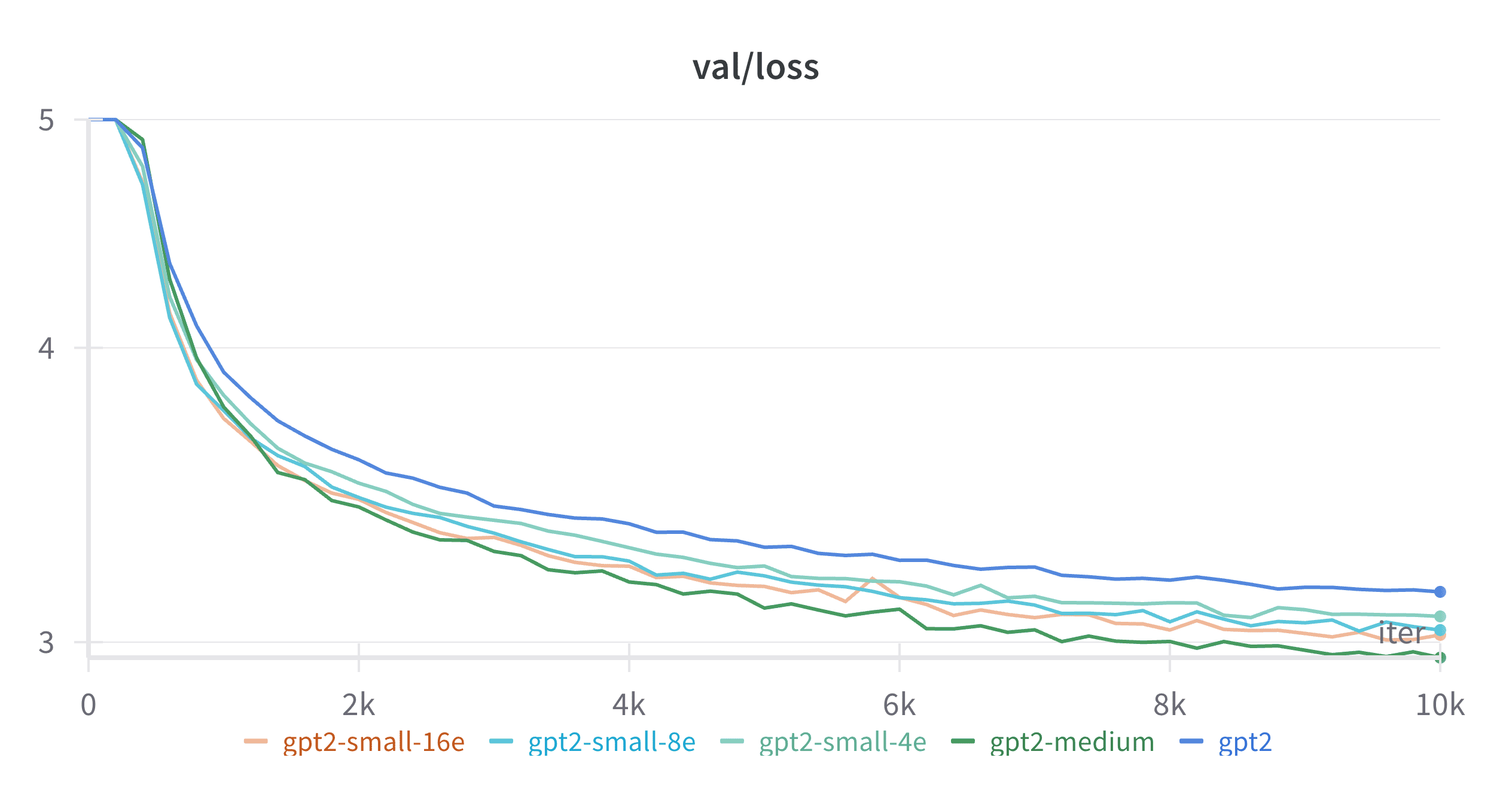
Figure 3: Performance scaling of GPT2-MoE models with increasing expert count
From Figure 2 (from the original Switch Transformers paper), you can see how scaling T5-base to 16, 32, 64, and 128 experts leads to corresponding performance gains. My experiments, shown in Figure 3, tell the same story – the loss curves get progressively lower as we add more experts to GPT2-small. While the metrics differ between the two plots (negative log perplexity vs. raw loss), the trend is identical: more experts yield better performance at the same computational cost.
2. MoE models achieve comparable performance to larger dense models with significantly lower FLOPS
![]()
Figure 4: Switch Transformer with the same FLOPS as T5-base matches the performance of T5-large (3.5x the FLOPS of T5-base)
Another compelling insight from the Switch Transformer paper is that a computationally-equivalent MoE model substantially outperforms its dense counterpart. As demonstrated in Figure 4 above, a model using T5-base architecture with 64 MoE experts not only surpasses T5-base itself but can match the performance of T5-large – which requires 3.5x the computational resources.
My experiments with GPT-2 show similar results. In Figure 3, you can see that as we increase the number of experts, our MoE variants of GPT2-small approach the performance of GPT2-medium (which requires 3.5x the FLOPS of GPT2-small). While my largest experiment with 16 experts doesn’t quite reach GPT2-medium performance levels, the trend is clear. Extrapolating from these results, we can reasonably predict that scaling to 32 or 64 experts would likely match or exceed GPT2-medium’s performance – all while maintaining the computational efficiency of the smaller model.
3. MoE models require significantly more parameters than dense models for equivalent performance
A corollary to point #2 is that when comparing models with similar parameter counts (rather than FLOPS), MoE models actually underperform their dense counterparts by a substantial margin. As Figure 3 and the table below demonstrate, even though GPT-2 small with 8 and 16 experts has more parameters than GPT-2 medium, it still doesn’t match the dense model’s performance:
| Model | Parameters | Val loss after 10k steps |
|---|---|---|
| GPT-2 Small | 124M | 3.151 |
| GPT-2 Small 4e | 293M | 3.076 |
| GPT-2 Small 8e | 520M | 3.036 |
| GPT-2 Small 16e | 973M | 3.021 |
| GPT-2 Medium | 353M | 2.955 |
This raises an interesting question: how many parameters would an MoE model need to match a dense model’s performance? Using the findings from the Switch Transformer paper (where T5-base with 64 experts matches T5-large’s performance), we can estimate that it would take GPT2-small with 64 experts to match GPT2-medium’s performance. That would translate to approximately 3.6B parameters - an order of magnitude more than GPT2-medium’s 353M parameters.
This highlights the fundamental trade-off of MoE architectures: they offer remarkable computational efficiency but require substantially more parameters to achieve the same performance as dense models. This parameter inefficiency is the price we pay for the computational benefits - a worthwhile exchange in many practical scenarios where inference costs or latency are primary concerns.
4. MoE models can be scaled by increasing the number of active experts per token
Previously, we discussed how MoE architecture decouples the number of model parameters from the model FLOPS, showing that we can scale performance by increasing the number of experts while keeping FLOPS constant. But can we do the reverse - scale MoE by increasing the model FLOPS while keeping the number of parameters the same? It turns out we can.
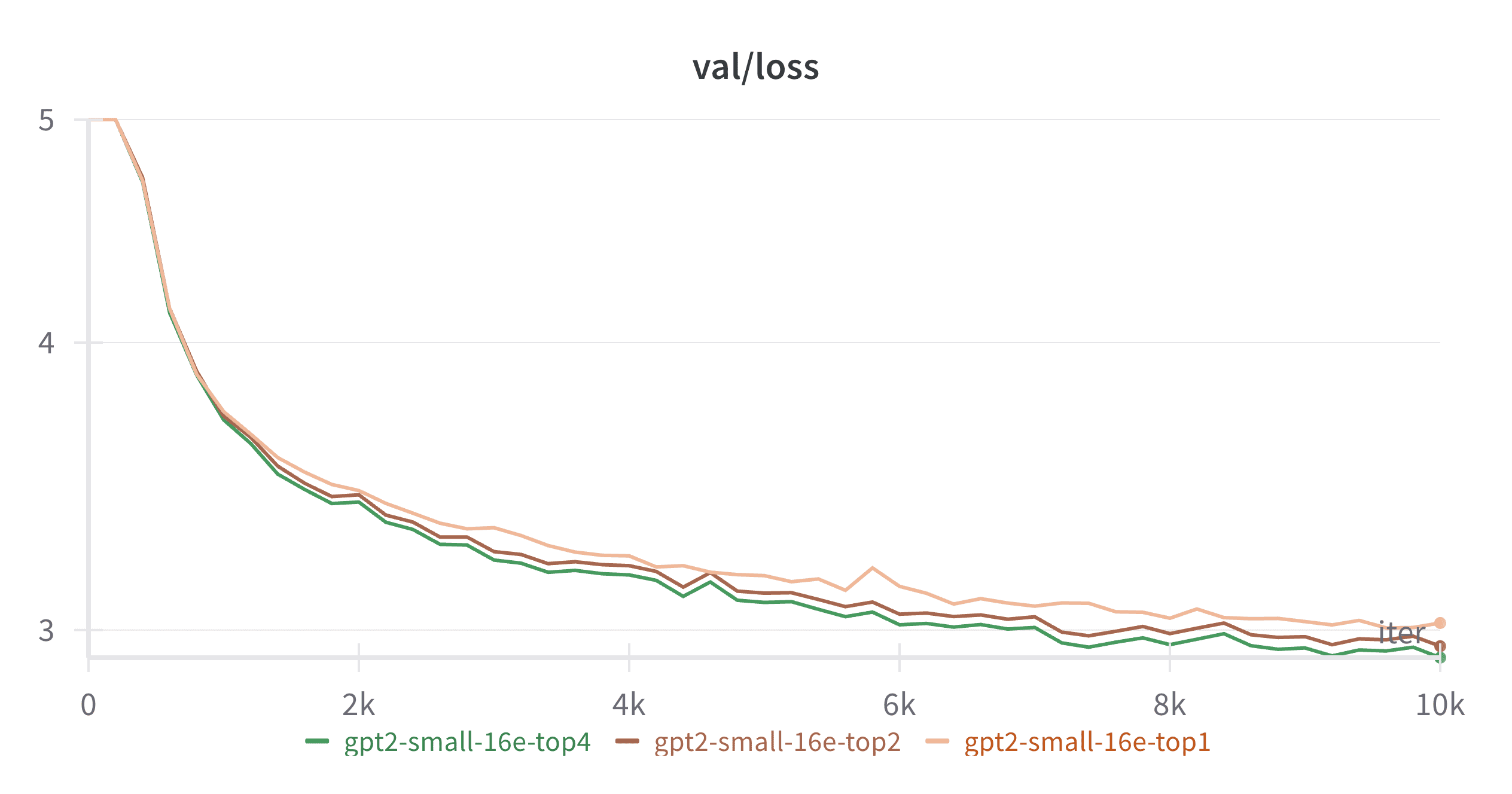
Figure 5: MoE models can also be scaled by increasing top-k, the number of active experts for any given token
As shown in Figure 5, by increasing top-k (the number of activated experts per token), we effectively increase the model’s forward pass FLOPS (a.k.a. active parameters) and achieve clear performance gains. Importantly, the total number of model parameters remains unchanged throughout these experiments, as all variants maintain 16 experts. This reveals one of the most powerful aspects of MoE architecture: it provides two independent scaling axes:
- Total parameter count: Scaled by increasing the number of experts
- Active parameter count (FLOPS): Scaled by increasing top-k, the number of experts activated per token
5. Expert Load Balancing: A Critical Component for Training Effective MoE Models
One crucial aspect of training MoE models effectively is ensuring balanced utilization across all experts. Without proper load balancing, some experts might become under-utilized or entirely “dead,” while others become overloaded. This imbalance can significantly degrade model performance and negate the benefits of the MoE architecture.
I implemented a load balancing loss similar to the one described in the Switch Transformer paper, with some generalizations to handle top-k expert selection (rather than just the top-1 approach in the original paper):
\[loss = \alpha \cdot N \cdot \sum_{i=1}^N f_{i} \cdot P_{i}\]Where:
- $p_{i}(x)$ is the probability of routing token $x$ to expert $i$
- $f_i$ is the fraction of tokens dispatched to expert $i$ considering top-k filtering
- $P_i$ is the fraction of the router probability allocated for expert $i$ across all tokens in the batch $\mathcal{B}$
These components are calculated as:
\[f_i = \frac{1}{T} \sum_{x \in \mathcal{B}} \mathbb{1}\{ i \in \text{top-}k(p(x)) \}\] \[P_i = \frac{1}{T} \sum_{x \in \mathcal{B}} p_{i}(x)\]This formulation generalizes the load balance loss from Switch Transformers, extending it beyond just the top-1 (argmax) expert to handle any top-k selection strategy.
Here’s the implementation:
def expert_load_balance_loss(router_logits, num_experts: int, top_k: int) -> torch.Tensor:
    """
    Computes the auxiliary load balancing loss as described in the Switch Transformers paper.

    This loss encourages a balanced assignment of tokens to experts by penalizing
    scenarios where some experts process significantly more tokens than others.

    Args:
        router_logits: A tuple of router logits from each layer,
                       each with shape [batch_size * seq_length, num_experts]
        num_experts: Total number of experts in the model
        top_k: Number of experts selected for each token

    Returns:
        torch.Tensor: The computed load balancing loss
    """
    # Move all router logits to the same device and concatenate
    compute_device = router_logits[0].device
    concatenated_router_logits = torch.cat(
        [layer_gate.to(compute_device) for layer_gate in router_logits], dim=0
    )

    # Convert logits to probabilities
    routing_weights = torch.nn.functional.softmax(concatenated_router_logits, dim=-1)

    # Select top-k experts for each token
    _, selected_experts = torch.topk(routing_weights, top_k, dim=-1)

    # Create a one-hot encoding of which experts are selected for each token
    expert_mask = torch.nn.functional.one_hot(selected_experts, num_experts)

    # Calculate the fraction of tokens assigned to each expert
    tokens_per_expert = torch.mean(expert_mask.float(), dim=0)

    # Compute the average routing probability for each expert
    router_prob_per_expert = torch.mean(routing_weights, dim=0)

    # The auxiliary loss is the product of these two quantities, summed over all experts
    # Scaled by num_experts to keep the loss magnitude consistent regardless of expert count
    overall_loss = torch.sum(tokens_per_expert * router_prob_per_expert.unsqueeze(0))

    return overall_loss * num_experts
Visualize the Load Balance Loss
All those formulas and code might seem abstract, so let’s visualize what different load balancing scenarios actually look like and how they affect the loss value. The following examples are based on a model with 8 experts and top-1 routing:
| Situation | Visualization | Loss |
|---|---|---|
| Perfectly balanced experts | 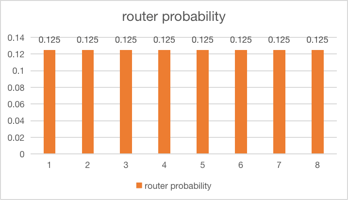 |
$loss = 8 \times \sum_{i=1}^8 \frac{1}{8} \cdot \frac{1}{8} = 1$ |
| All tokens go to 1 expert | 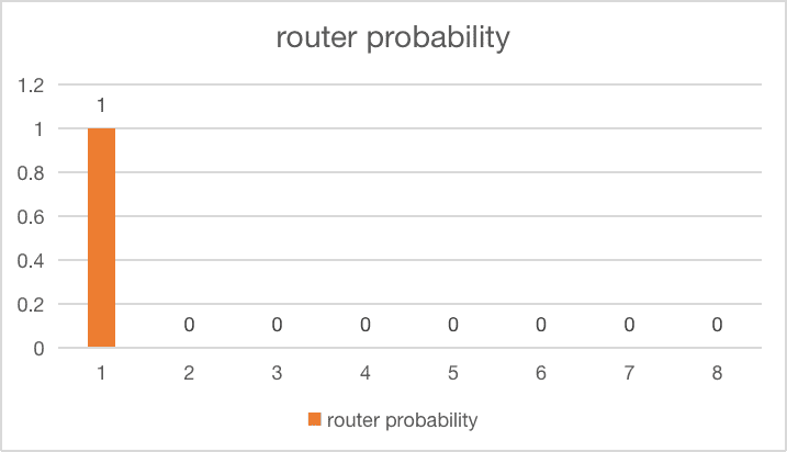 |
$loss = 8 \times 1 \times 1 = 8$ |
| 1 expert gets dropped completely | 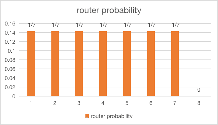 |
$loss = 8 \times \sum_{i=1}^7 \frac{1}{7} \cdot \frac{1}{7} = 1.1428$ |
| 2 experts get dropped completely | 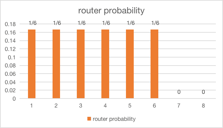 |
$loss = 8 \times \sum_{i=1}^6 \frac{1}{6} \cdot \frac{1}{6} = 1.3333$ |
| 2 experts get slightly unbalanced | 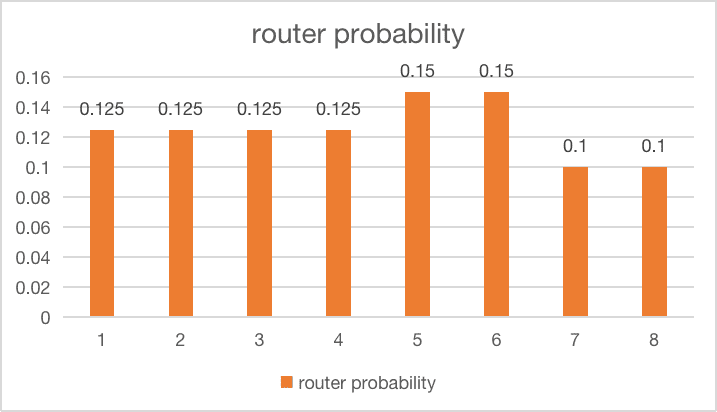 |
$loss = 8 \times (0.125^2 \times 4 + 0.15^2 \times 2 + 0.1^2 \times 2) = 1.02$ |
| 4 experts get slightly unbalanced | 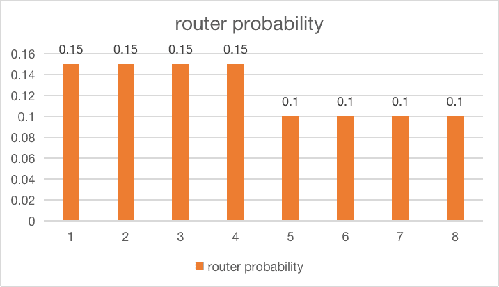 |
$loss = 8 \times (0.15^2 \times 4 + 0.1^2 \times 4) = 1.04$ |
These visualizations illustrate how the loss function penalizes different types of imbalance:
-
The worst case is when all tokens are routed to a single expert (loss = 8), effectively negating the benefits of having multiple experts.
-
When experts are perfectly balanced, we achieve the minimum loss value (loss = 1).
-
Having a few completely dropped experts incurs a relatively significant penalty.
-
Slight imbalances across multiple experts result in only minor increases to the loss, showing that the function is primarily designed to prevent extreme cases of imbalance rather than enforcing perfect uniformity.
Load Balance Loss Keeps the Balance
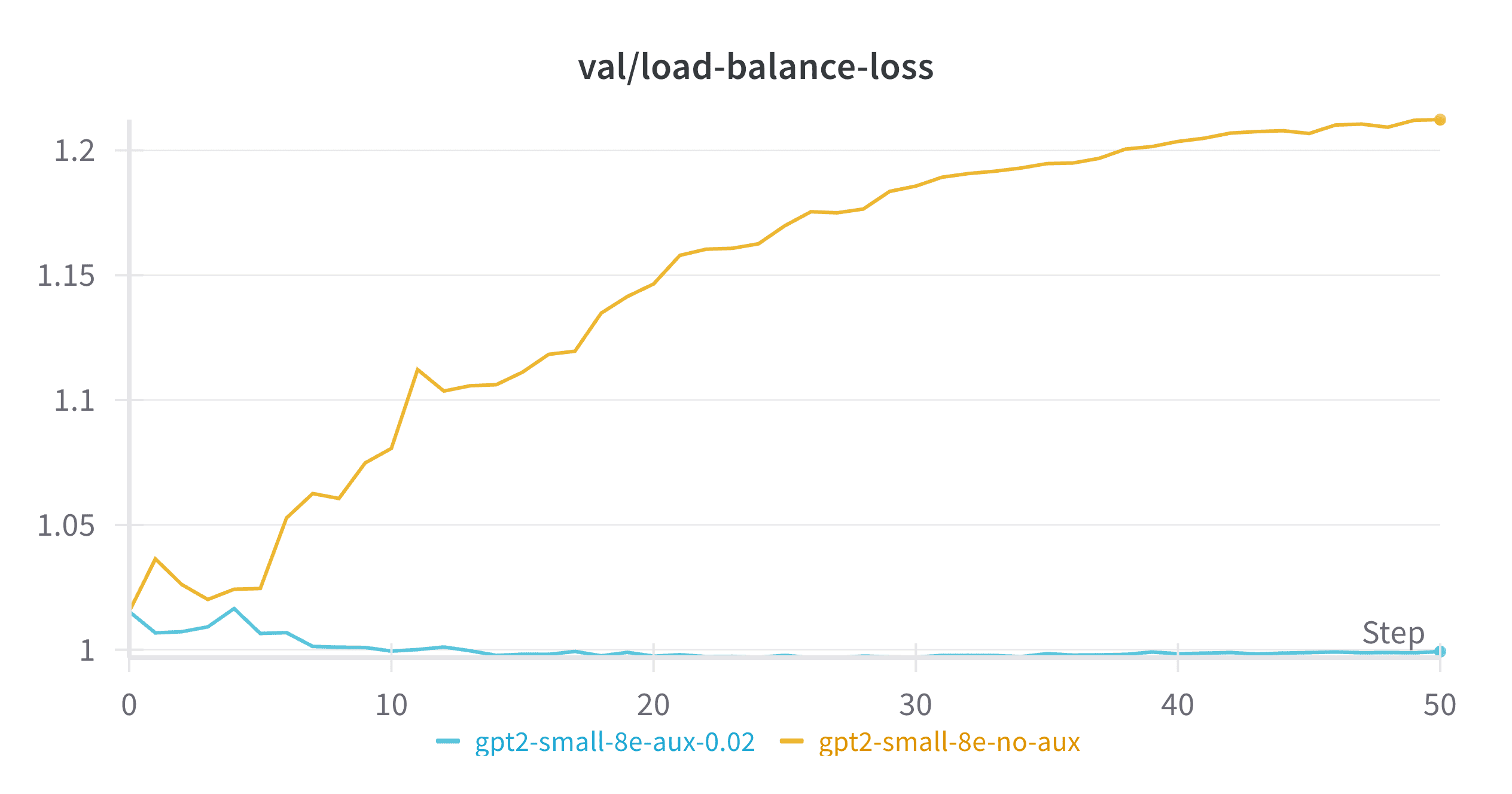
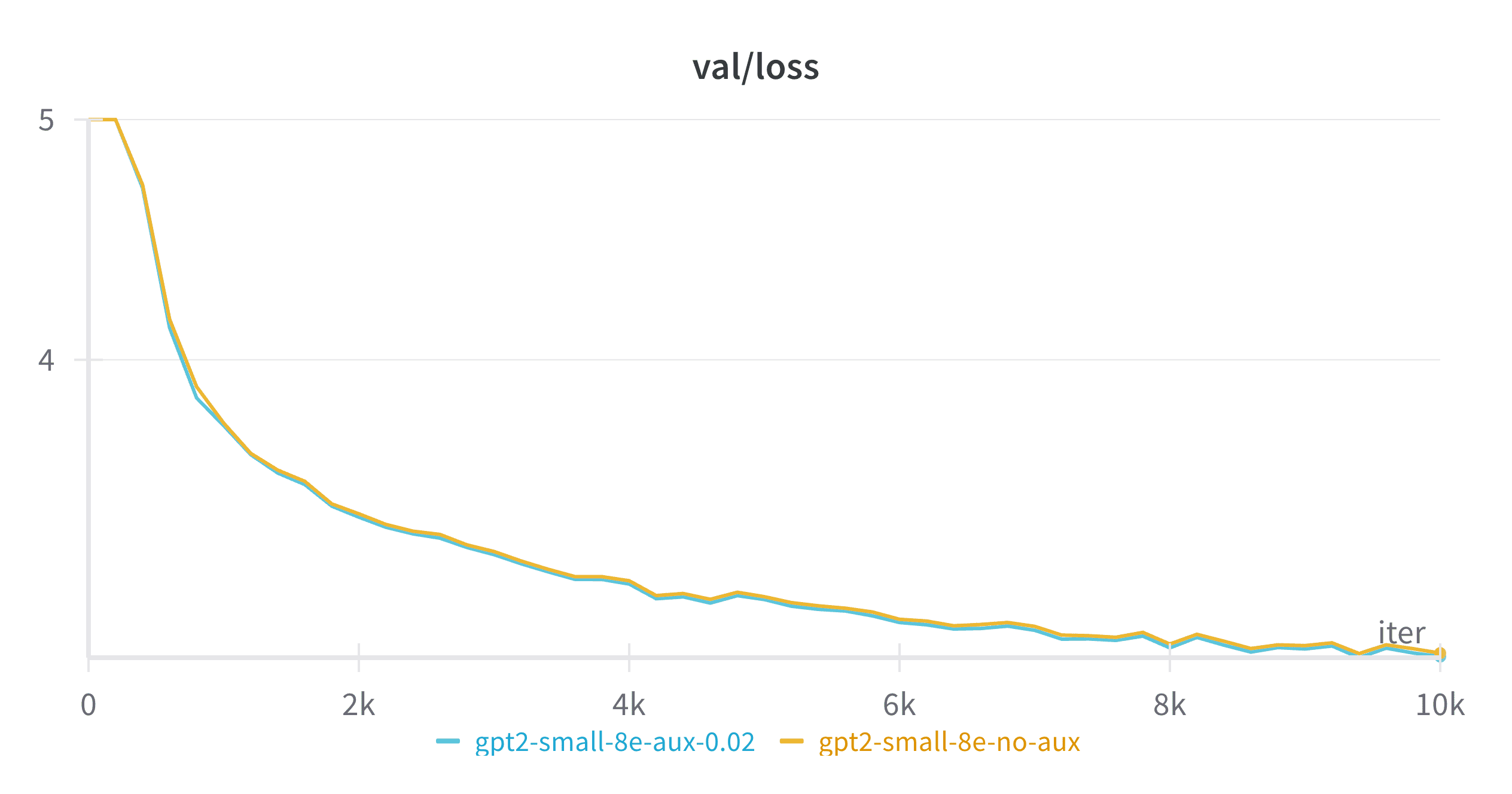
Figure 6: Load Balance Loss and Language Model Loss of the same MoE model with different auxiliary loss coefficients
As shown in Figure 6, experts naturally start in a balanced state at initialization (when router weights are random and statistically balanced). However, the trajectory diverges dramatically depending on whether we apply the auxiliary loss. When the auxiliary loss coefficient ($\alpha$) is set to 0 (effectively turning it off), the load balance loss steadily increases to around 1.2 as training progresses. Comparing this with our visualizations above, a load balance loss of 1.2 corresponds to dropping approximately 1-2 out of the 8 experts! In contrast, the model with auxiliary loss enabled maintains remarkable stability, hovering close to the theoretical minimum of 1.
Surprisingly, the impact on actual language modeling performance is relatively subtle - the model with imbalanced experts only slightly underperforms the balanced model (with a loss gap of around 0.01, barely visible on the chart). This suggests that losing a small percentage of experts only marginally decreases the performance ceiling, as long as the resulting imbalance remains stable over time. While not ideal, a model effectively using 7 experts performs quite similarly to one using all 8 experts.
Suprisingly, when it comes to Language Model Loss, the model with imbalanced experts only slightly underforms the model with balanced experts (the loss gap is around 0.01 and barely visible). My hypothesis is that dropping a small percentage of the experts only slightly decrease the performance celling of the model, as long as the expert imbalance is stable. Although not ideal, a model with 7 experts’s performance is quite close to a model with 8 experts.
Loss Spikes: The Real Threat to MoE Training Stability
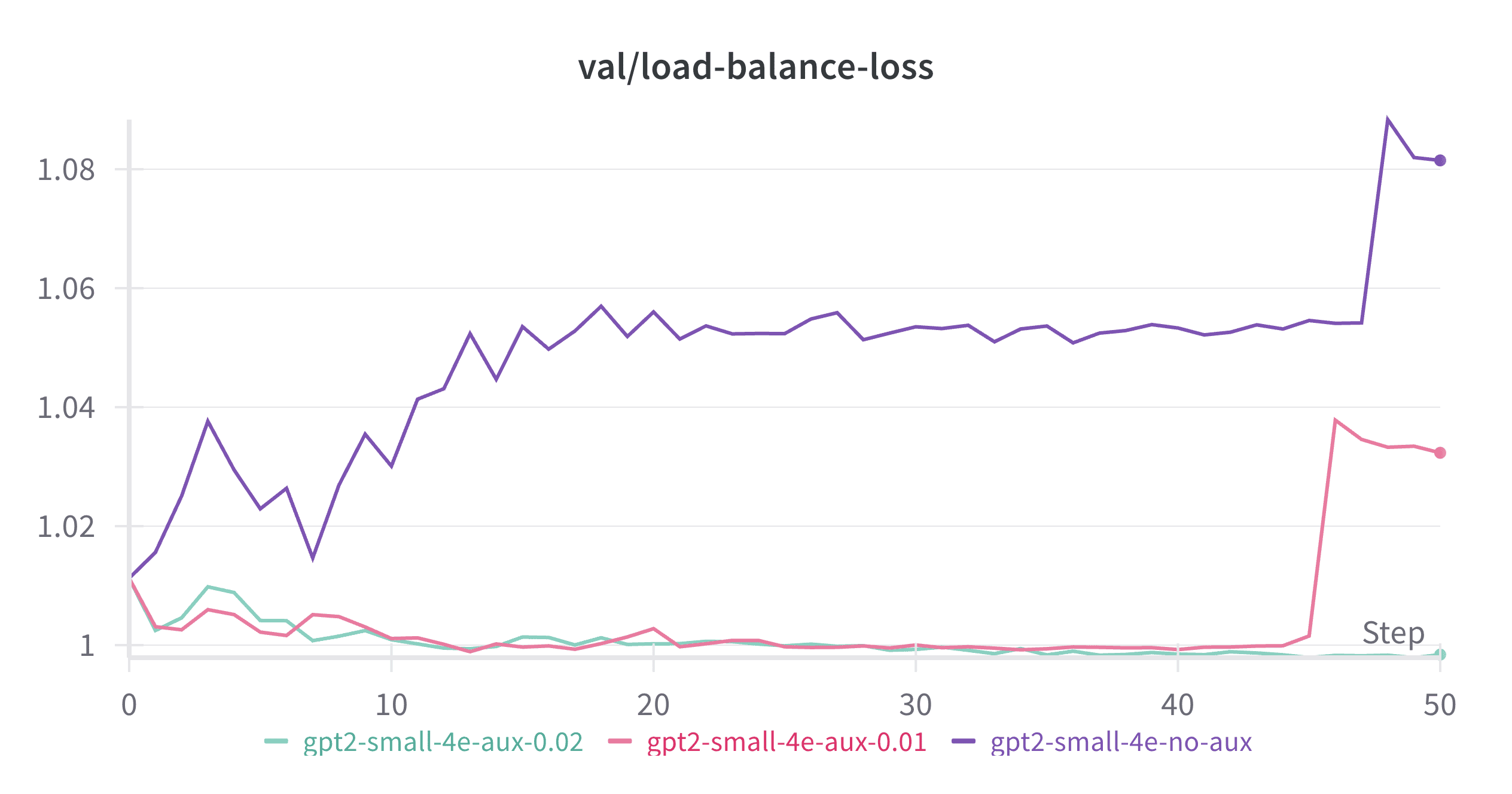
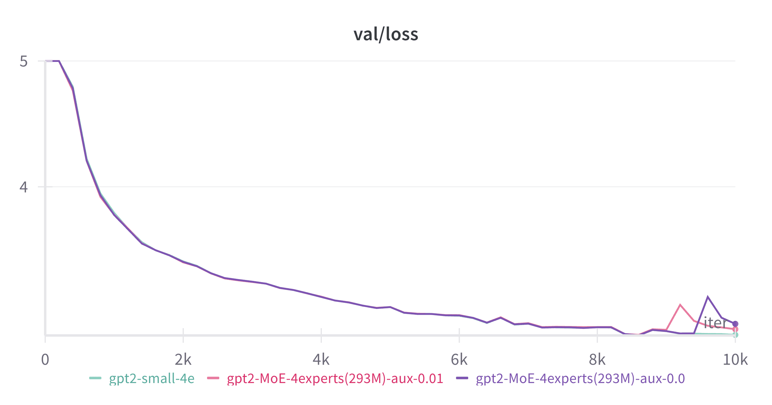
Figure 7: Auxiliary loss helps control spikes in both load balance loss and language model loss
If stable but imbalanced expert utilization isn’t the primary source of MoE training instability, then what is? My experiments point to sudden spikes in load balance loss and the resulting spikes in language model loss as the main culprit.
My hypothesis is that these spikes occur when a set of tokens abruptly switches from one expert to another after a gradient update, disrupting the previously stable routing patterns. The newly assigned expert hasn’t previously encountered these tokens and consequently produces high language model loss. This issue is particularly problematic with top-1 routing, where each token is assigned to exactly one expert that bears full responsibility for it. The problem could be mitigated by setting top-k greater than 1, distributing the responsibility across multiple experts.
This phenomenon becomes especially detrimental in later stages of training, when each expert has already adapted to a specific data distribution. At that point, it takes significant time for experts to update their weights to accommodate a new set of tokens with different characteristics.
As demonstrated in Figure 7, increasing the auxiliary loss coefficient progressively reduces the frequency and magnitude of these spikes. With $\alpha = 0.02$, we observe almost no spikes at all, resulting in much smoother and more stable training.
Conclusion
Through this nanoMoE project, I’ve explored the Mixture of Experts architecture by extending NanoGPT, gaining practical insights that align with existing research.
My experiments suggest several interesting observations about MoE models:
- They allow parameter scaling while keeping computation relatively constant
- They can achieve performance comparable to denser models with lower computational requirements
- They tend to require more total parameters than dense models for equivalent performance
- They offer flexibility through dual-axis scaling (total experts and active experts per token)
- Proper load balancing appears important for training stability, especially for preventing disruptive routing shifts
As the field has increasingly embraced MoE architectures for their efficiency advantages, implementations like nanoMoE can help practitioners better understand the underlying mechanisms (as it has certainly helped me). Even these modest experiments reveal some of the trade-offs and design considerations that make MoE models an important part of the current language model landscape.
For those interested in exploring further, the complete code for this project is available on GitHub.