Conditional Random Field (CRF) is a probabilistic graphical model that excels at modeling and labeling sequence data with wide applications in NLP, Computer Vision or even biological sequence modeling. In ICML 2011, it received “Test-of-Time” award for best 10-year paper, as time and hindsight proved it to be a seminal machine learning model. It is a shame that I didn’t know much about CRF till now but better late than never!

Reading summaries of the following paper:

• Original paper: Conditional Random Fields: Probabilistic Models for Segmenting and Labeling Sequence Data
• Tutorial from original author of CRF: Intro to Conditional Random Fields
• Technique for confidence estimation for entities: Confidence estimation for information extraction

1. Hidden Markov Model (HMM)

Hidden Markov Model (HMM) models a sequence of observations $X = \{x_t \}{t=1}^T$ by assuming that there is an underlying sequence of states (also called hidden states) $Y = \{y_t \}{t=1}^T$ drawn from a finite state $S$. HMM is powerful because it models many variables that are interdependent sequentially. Some typical tasks for HMM is modeling time-series data where observations close in time are related, or modeling natural languages where words close together are interdependent.

In order to model the joint distribution $p(Y, X)$ tractably, HMM makes two strong independence assumptions:

• Markov property: each state $y_t$ depends only on its immediate predecessor $y_{t-1}$ and independent of all its ancestors $y_{t-2}, \cdots y_{1}$.
• Output independence: each observation $x_t$ depends only on the current state $y_t$

With these assumptions, wen can model the joint probability of a state sequence $Y$ and an observation sequence $X$ as

\[p(Y, X) = \prod_{t=1}^T p(y_t \vert y_{t-1}) p(x_t \vert y_t)\tag{1}\]

where the initial state distribution $p(y_1)$ is written as $p(y_1 \vert y_0)$.

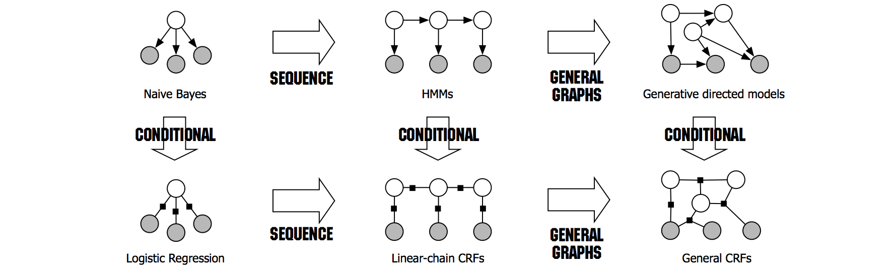
2. Generative vs Discriminative Models

Generative models learn a model of the joint probability $p(y,x)$ of the inputs $x$ and labels $y$. HMM is an generative model. Modeling the joint distribution is often difficult since it requires modeling the distribution $p(x)$, which can include complex dependencies. A solution is to use discriminative models to directly model the conditional distribution $p(y \vert x)$. With this approach, dependencies among the input variables $x$ do not need to be explicitly represented, affording the use of rich, global features of the input.

An interesting read about this topic is On Discriminative & Generative Classifiers: A comparison of logistic regression and naive Bayes from the famous Prof. Andrew Ng back when he was a graduate student. A generative model and a discriminative model can form a Generative-Discriminative pair if they are in the same hypothesis space. For example,

• if $p(x \vert y)$ is Gaussian and $p(y)$ is multinomial, then Linear Discriminant Analysis and Logistic Regression models the same hypothesis space
• if $p(x \vert y)$ is Gaussian and $p(y)$ is binary, then Gaussian Naive Bayes has the same model form as Logistic Regression
• There is a discriminative analog to HMM, and it’s the linear-chain Conditional Random Field (CRF).

3. Linear-Chain Conditional Random Field

From HMM to CRF

To motivate the comparison between HMM and CRF, we can re-write the Eq. (1) in a different form

\[p(Y, X) = \frac{1}{Z} \prod_{t=1}^T \text{exp} \left\{ \sum_{k = 1}^K \lambda_k f_k \left( y_t, y_{t-1}, x_t \right) \right\}\tag{2}\]

The $K$ feature function $f_k\left( y_t, y_{t-1}, x_t\right)$ are a general form that takes into account of all state transitions probabilities and state-observation probabilities. There is one feature function $f_{ij}( y, y’, x) = \boldsymbol{1}{y =i} \boldsymbol{1}{y’ =j}$ for each state transition pair $(i,j)$ and one feature function $f_{io}( y, y’, x) = \boldsymbol{1}{y=i} \boldsymbol{1}{x=0}$ for each state-observation pair $(i,o)$. Z is a normalization constant for the probability to sum to 1.

To turn the above into a linear-chain CRF, we need to write the conditional distribution

\[\begin{align} p(Y \vert X) &= \frac{p(Y, X)}{\sum_Y p(Y, X)} \\\\ &= \frac{\prod_{t=1}^T \text{exp} \left\{ \sum_{k = 1}^K \lambda_k f_k\left( y_t, y_{t-1}, x_t\right) \right\} }{\sum_{y'} \prod_{t=1}^T \text{exp} \left\{ \sum_{k = 1}^K \lambda_k f_k\left( y'_t, y'_{t-1}, x_t\right) \right\}} \\\\ &= \frac{1}{Z(X)} \prod_{t=1}^T \text{exp} \left\{ \sum_{k = 1}^K \lambda_k f_k\left( y_t, y_{t-1}, x_t\right) \right\} \end{align} \tag{3}\]

Parameter Estimation

Just like most other machine learning models, the parameter is estimated via Maximum Likelihood Estimation (MLE). The objective is to find the parameter that maximize the conditional log likelihood $l(\theta)$

\[\begin{align} l(\theta) &= \sum_{i=1}^N \ \text{log} p(y^{(i)} \vert x^{(i)}) \\\\ &= \sum_{i=1}^N \sum_{t=1}^T \sum_{k=1}^K \lambda_k f_k\left( y_t^{(i)}, y_{t-1}^{(i)}, x_t^{(i)}\right) - \sum_{i=1}^N \text{log} Z(x^{(i)}) \end{align} \tag{4}\]

The objective function $(\theta)$ cannot be maximized in closed form, so numerical optimization is needed. The partial derivative of Eq. (4) is

\[\frac{\partial l(\theta)}{\partial \lambda_k} = \sum_{i=1}^N \sum_{t=1}^T f_k\left( y_t^{(i)}, y_{t-1}^{(i)}, x_t^{(i)}\right) - \sum_{i=1}^N \sum_{t=1}^T \sum_{y'_{t-1}, y'_{t}} f_k\left( y'_{t}, y'_{t-1}, x_t^{(i)}\right) p(y'_{t}, y'_{t-1} \vert x_t^{(i)}) \tag{5}\]

which has the form of (observed counts of $f_k$) - (expected counts of $f_k$). To compute the gradient, inference is required to compute all the marginal edge distributions $p(y’{t}, y’{t-1} \vert x_t^{(i)})$. Since the quantities depend on $x^{(i)}$, we need to run inference once for each training instance every time the likelihood is computed.

Inference

Before we go over the typical inference tasks for CRF, let’s define a shorthand for the weight on the transition from state $i$ to state $j$ when the current observation is $x$.

\[\begin{align} \Psi_t(j,i,x) &= p(y_{t} = j \vert y_{t-1} = i) \cdot p(x_{t} = x \vert y_{t} = j) \\\\ &= \left[ \delta_{t}(i) \ \text{exp} \left( \sum_{k = 1}^K \lambda_k f_k\left( j, i, x_{t+1}\right) \right) \right] \end{align} \tag{6}\]

Most probable state sequences

The most needed inference task for CRF is to find the most likely series of states $Y^{*} = \text{argmax}_{Y} \ p(Y \vert X)$, given the observations. This can be computed by the Viterbi recursion. The Viterbi algorithm stores the probability of the most likely path at time $t$ that accounts for the first $t$ observations and ends in state $j$.

\[\delta_{t}(j) = \text{max}_{i \in S} \ \delta_{t-1}(i) \cdot \Psi_t(j,i,x) \tag{7}\]

The recursive formula terminates in $p^{*} = \text{argmax}{i \in S} \ \delta{T}(i)$. We can backtrack through the dynamic programming table to find the mostly probably state sequences.

Probability of an observed sequence

We can use Eq. (3) to compute the likelihood of an observed sequence $p(Y \vert X)$. While the numerator is easy to compute, the denominator $Z(X)$ is very difficult to compute since it contains an exponential number of terms. Luckily, there is another dynamic programming algorithms called forward-backward to compute it efficiently.

The idea behind forward-backward is to compute and store two sets of variables, each of which is a vector with size as the number of states. The forward variables $\alpha_t(j) = p(x_1, \cdots, x_t, y_t = j)$ stores the probability of all the paths through the first $t$ observations and ends in state $j$. The backward variables $\beta_t(i) = p(x_t, \cdots, x_T, y_t = i)$ is the exact reverse and stores the probability of all the paths through the last $T-t$ observations with the t-th state as $i$

\(\alpha_t(j) = \sum_{i \in S} \Psi_{t}(j, i, x_t) \alpha_{t-1}(i)\tag{8}\) \(\beta_t(i) = \sum_{j \in S} \Psi_{t+1}(j, i, x_t) \beta_{t+1}(j)\tag{9}\)

The initialization for the forward-backward is $\alpha_1{j} = \Psi_{t}(j, y_0, x_1)$ and $\beta_T(i) = 1$. After the dynamic programming table is filled, we can compute $Z(X)$ as

\[Z(x) = \sum_{i \in S} \alpha_T(i)\tag{10}\]

Forward-backward algorithm is also used to compute all the marginal edge distributions $p(y_{t}, y_{t-1} \vert x_t)$ in Eq. (5) that is needed for computing the gradient.

\[p(y_{t}, y_{t-1} \vert x_t) = \alpha_{t-1}(y_{t-1}) \Psi_t(y_{t},y_{t-1},x_t) \beta_t(y_t)\]

Confidence in predicted labeling over a specific segment

Sometimes in task like Named Entity Recognition (NER), we are interested in the model’s confidence in its predicted labeling over a segment of input to estimate the probability that a field is extracted correctly. This marginal probability $p(y_t, y_{t+1}, \cdots, y_{t+k} \vert X)$ can be computed using constrained forward-backward algorithm, introduced by Culotta and McCallum.

The algorithm is an extension to the forward-backward we described above, but with added constraints such that each path must conforms to some sub-path of constraints $C = \{ y_t, y_{t+1}, \cdots\}$. $y_t$ can either be a positive constraint (sequence must pass through $y_t$) or a negative constraint (sequence must not pass through $y_t$). In the context of NER, the constraints $C$ corresponds to an extracted field. The positive constraints specify the tokens labeled inside the field, and the negative field specify the field boundary.

The constraints is a simple trick to shut off the probability of all paths that don’t conform to the constraints. The calculation of the forward variables in Eq. (8) can be modified slightly to factor in the constraints

\[\alpha'_t(j) = \begin{cases} \sum_{i \in S} \Psi_{t}(j, i, x_t) \alpha_{t-1}(i), & \text{if} \ j \ \text{conforms to} \ y_{t} \\\\ 0, & \text{otherwise} \end{cases}\]

For time steps not constrained by $C$, Eq. (8) is used instead. Similar to Eq. (10), we calculate the probability of the set of all paths that conform to $C$ as $Z’(X) = \sum_{i \in S} \alpha’_T(i)$. The marginal probability can be computed by replacing $Z(X)$ with $Z’(X)$ in Eq. (3).