Batch Normalization, Layer Normalization and Why They Work

Reading notes / survey of three papers related to Batch Normalization

• Batch Normalization: Accelerating Deep Network Training by Reducing Internal Covariate Shift, the paper that introduced Batch Normalization, one of the breakthroughs in Deep Learning
• Layer Normalization that extended Batch Normalization to RNNs
• How Does Batch Normalization Help Optimization?(No, It Is Not About Internal Covariate Shift), a paper (barely one week old at the time of writing) that dived into the fundamental factors for Batch Normalization’s success empirically and theoretically

1. Why Normalization?

Covariate Shift

Covariate Shift refers to the change in the distribution of the input variables $X$ between a source domain $\mathcal{s}$ and a target domain $\mathcal{t}$. We assume $P_{\mathcal{s}}(Y \vert X) = P_{\mathcal{t}}(Y \vert X)$ but a different marginal distribution $P_{\mathcal{s}}(X) \neq P_{\mathcal{t}}(X)$.

We are interested in modeling $P(Y \vert X)$. However, we can only observe $P_{\mathcal{s}}(Y \vert X)$. The optimal model for source domain $\mathcal{s}$ will be different from the optimal model for target domain $\mathcal{t}$. The intuition, as shown in the diagram below, is that the optimal model for $P_{\mathcal{s}}(X)$ will put more weights and perform better in dense area of $P_{\mathcal{s}}(X)$, which is different from the dense area of $P_{\mathcal{t}}(X)$.

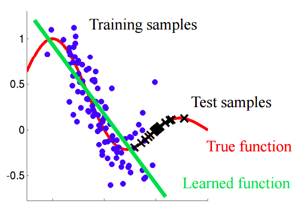
Covariate Shift Diagram Source

Internal Covariate Shift (ICS)

In Neural Networks (NN), we face a similar situation like Covariate Shift. A layer $l$ in a vanilla feedforward NN can be defined as

where $X^{l-1}$ is $m \times n_{in}$ and $W^{l}$ is $n_{in} \times n_{out}$. $m$ is the number of samples in the batch. $n_{in}$ and $n_{out}$ are the input and output feature dimension of the layer.

The weights $W^{l}$ is learned to approximate $P_{\mathcal{s}}(X^{l} \vert X^{l-1})$. However, the input from last layer $X^{l-1}$ is constantly changing so $W^{l}$ needs to continuously adapt to the new distribution of $X^{l-1}$. Ioffe et al. defined such change in the distributions of internal nodes of a deep network during training as Internal Covariate Shift.

2. Batch Normalization (BN)

An obvious procedure to reduce ICS is to fix the input distribution to each layer. And that is exactly what Ioffe et al. proposed. Batch Normalization (BN) is a layer that normalizes each input feature to have mean of 0 and variance of 1. For a BN layer with $d$-dimensional input $X = (x^{1}, \cdots, x^{d})$, each feature is normalized as

Mini Batch Statistics

Computing the mean and standard deviation of each feature requires iterating through the whole dataset, which is impractical. Thus, $\mu_{x^{(k)}}$ and $\sigma_{x^{(k)}}$ are estimated using the empirical samples from the current batch.

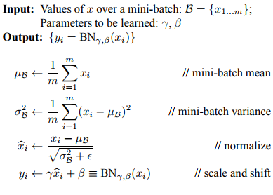
Scale and Shift Parameters

To compensate for the loss of expressiveness due to normalization, a pair of parameters $\gamma^{(k)}$ and $\beta^{(k)}$ are trained to scale and shift the normalized value.

The scale and shift parameters restore the representation power of the network. By setting $\beta^{(k)} = \mu_{x^{(k)}}$ and $\gamma^{(k)} = \sigma_{x^{(k)}}$, the original activations could be recovered, if that were the optimal thing to do.

PyTorch Implementation

class BatchNorm(nn.Module):
    def __init__(self, num_features, momentum=0.1, eps=1e-6):
        super(BatchNorm, self).__init__()
        self.num_features = num_features
        self.gain = nn.Parameter(torch.ones(num_features), requires_grad=True)
        self.bias = nn.Parameter(torch.zeros(num_features), requires_grad=True)
        self.momentum = momentum
        self.eps = eps
        self.initialized = False

    def forward(self, x):
        # x: [batch, num_feature, ?, ...]
        mean = torch.mean(x, dim=0, keepdim=True)  # [1, num_feature, ?, ...]
        var = torch.var(x, dim=0, unbiased=False, keepdim=True)  # [1, num_feature, ?, ...]
        if not self.initialized:
            self.register_buffer('running_mean', torch.zeros_like(mean))
            self.register_buffer('running_var', torch.ones_like(var))
            self.initialized = True
        if self.training:
            bn_init = (x - mean) / torch.sqrt(var + self.eps)
            self.running_mean = (1 - self.momentum) * self.running_mean + self.momentum * mean
            self.running_var = (1 - self.momentum) * self.running_var + self.momentum * var
        else:
            bn_init = (x - self.running_mean) / torch.sqrt(self.running_var + self.eps)
        return self.gain * bn_init + self.bias

Batch Normalization in Feed-forward NN

Consider the l-th hidden layer in a feed-forward NN. The summed inputs are computed through a linear projection with the weight matrix $W^l$ and the bottom-up inputs $X^l$. The summed inputs are passed through a BN layer and then an activation layer (whether to apply BN before or after the activation layer is a topic of debate), as following:

$Z^{l}$ is a

$Z^{l}$ is a $m \times n_{out}$ matrix, whose element $z_{ij}$ is the summed input to the j-th neuron from the i-th sample in the mini-batch.

Column j of $Z^{l}$ is the summed inputs to the j-th neuron from each m samples in the mini-batch. The BN layer is a whitening / column-wise normalization procedure to normalize $\left[ \textbf{z}{1}, \textbf{z}{2}, \cdots, \textbf{z}{n{out}}\right]$ to $\mathcal{N}(0,1)$. Each neuron/column has a pair of scale $\gamma$ and shift parameters $\beta$.

3. Layer Normalization (LN)

BN has had a lot of success in Deep Learning, especially in Computer Vision due to its effect on CNNs. However, it also has a few shortcomings:

• BN replies on mini-batch statistics and is thus dependent on the mini-batch size. BN cannot be applied to to online learning tasks (batch size of 1) or tasks that require a small batch size.
• There is no elegant way to apply BN to RNNs. Applying BN to RNNs requires computing and storing batch statistics for each time step in a sequence.

To tackle the above issues, Ba et al. proposed Layer Normalization(LN), a transpose of BN that computes the mean and variance used for normalization from all of the summed inputs to the neurons in a layer on a single training sample.

Using the same notation as above, we have $Z^{l}$ is a $m \times n_{out}$ matrix, whose element $z_{ij}$ is the summed input to the j-th neuron from the i-th sample in the mini-batch. Row i of $Z^{l}$ is the summed inputs to the all neuron in the l-th layer from the i-th sample in the mini-batch. As a direct transpose of BN, the LN layer is a row-wise normalization procedure to normalize $\left[ \textbf{z}{1}, \textbf{z}{2}, \cdots, \textbf{z}_{m}\right]$ to have mean zero and standard deviation of one. Same as BN, each neuron is given its own adaptive bias and scale parameters.

PyTorch Implementation

class LayerNorm(nn.Module):
	def __init__(self, num_features, eps=1e-6):
	    super(LayerNorm, self).__init__()
	    self.gain = nn.Parameter(torch.ones(num_features), requires_grad=True)  # [num_features]
	    self.bias = nn.Parameter(torch.zeros(num_features), requires_grad=True)  # [num_features]
	    self.eps = eps

	def forward(self, x):
	    # [?, ..., num_features]
	    mean = x.mean(-1, keepdim=True)
	    std = x.std(-1, keepdim=True)
	    return self.gain * (x - mean) / (std + self.eps) + self.bias

Layer Normalization on RNN

In RNN, the summed input are computed from the current input $\textbf{x}^t$ and previous hidden state $\textbf{h}^{t-1}$ as \(\textbf{a}^{(t)} = W_{hh}\textbf{h}^{(t-1)} + W_{xh}\textbf{x}^{(t)}\).

LN computes the layer-wise mean and standard deviation, then then re-centers and re-scales the activations \(\boldsymbol{\mu}^{(t)} =\frac{1}{H} \sum_{i=1}^H \textbf{a}^{(t)} \ \ \ \ \ \boldsymbol{\sigma}^{(t)} = \sqrt{\frac{1}{H} \sum_{i=1}^H (\textbf{a}^{(t)} - \boldsymbol{\mu}^{(t)})^2 } \ \ \ \ \ \textbf{h}^{(t)} = f \left( \frac{\boldsymbol{\gamma}}{\boldsymbol{\sigma}^{(t)}} \circ \left( \textbf{a}^{(t)} - \boldsymbol{\mu}^{(t)}\right) + \boldsymbol{\beta} \right)\)

LN provides the following benefits when applied to RNN:

• No need to compute and store separate running averages for each time step in a sequence because the normalization terms depend on only the current time-step.
• With LN, the normalization makes it invariant to re-scaling all of the summed inputs to a layer, which helps preventing exploding or vanishing gradients and results in much more stable hidden-to-hidden dynamics.

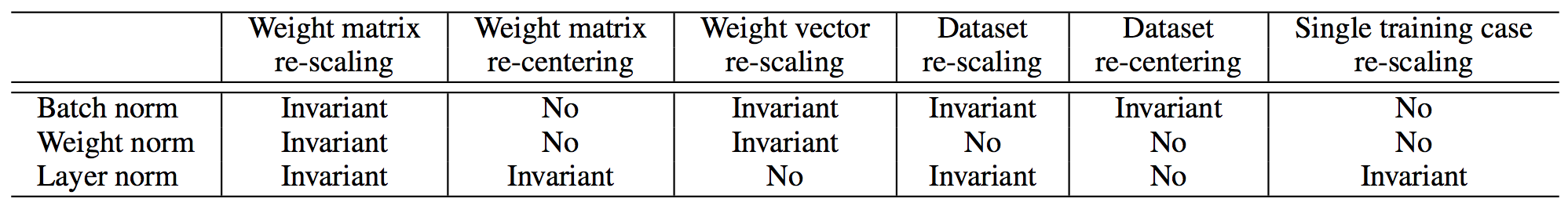
Invariance Properties of Normalizations

The below table shows the invariant properties of three different normalization procedures. These invariance properties make the training of the network more robust. Invariance to the scaling and shifting of weights means that proper weight initialization is not as important. Invariance to the scaling and shifting of data means that one bad (too big, too small, etc.) batch of input from the previous layer don’t ruin the training of next layer.

4. Not ICS, But A Smoother Optimization Landscape?

Despite its pervasiveness, the effectiveness of BN still lacks theoretical proof. Santurkar and Tsipras et al. recently proposed that ICS has little to do with the success of BN. Instead, BN makes the optimization landscape much smoother, which induces a more predictive and stable behavior of the gradients.

The performance of BN Doesn’t Stem From reducing ICS

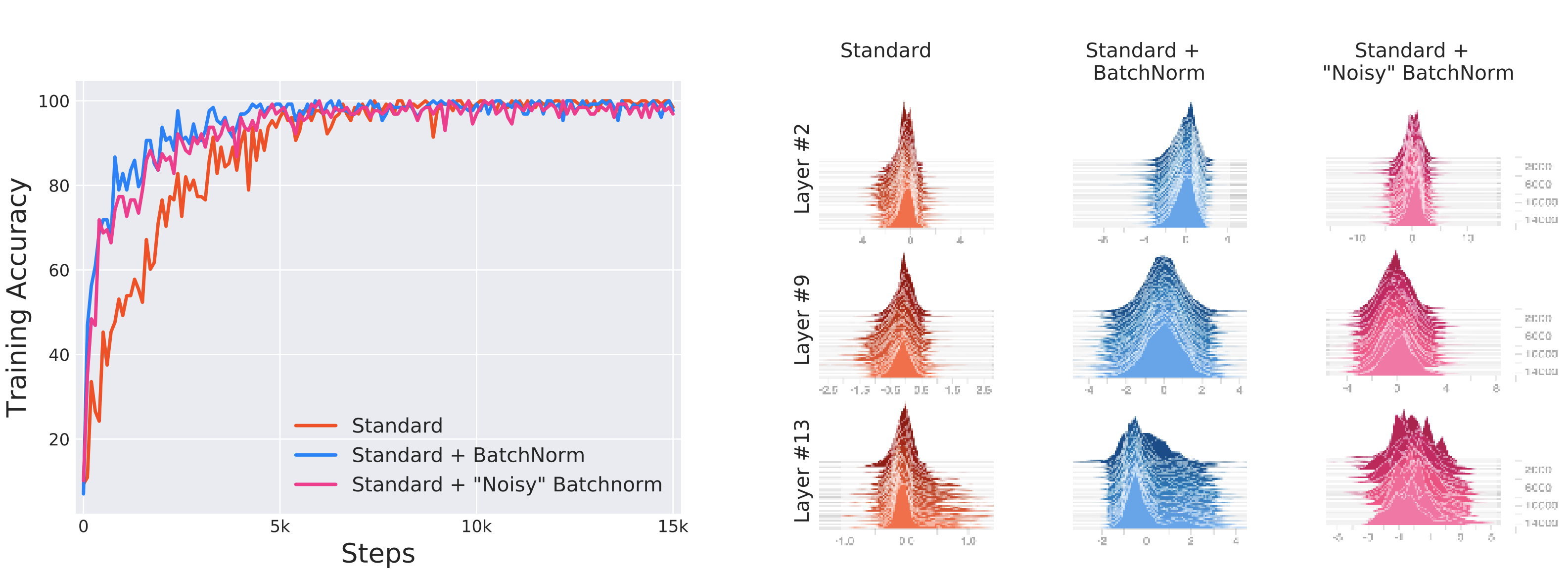
Santurkar and Tsipras et al. designed a clever experiment, where a network was trained with random noise (non-zero mean and non-unit variance distribution, changes at every time step) injected after BN layers, creating an artificial ICS. The performance of the network with “noisy” BN was compared with networks trained with and without BN. “Noisy” BN network has less stable distributions than the standard, no BN network due to the artificial ICS, yet it still performs better.

BN doesn’t even reduce ICS

Previously, ICS is a conception that has no measurement. Santurkar and Tsipras et al. defined a metric for ICS, which is difference （$ \vert \vert G_{t,i} - G_{t,i}^{\prime} \vert \vert_2$) between the gradient $G_{t,i}$ of the layer parameters and the same gradient $G_{t,i}^{\prime}$ after all the previous layers have been updated. Experiments showed that models with BN have similar, or even worse, ICS, despite performing better.

The Fundamental Phenomenon at Play: the Smoothing Effect

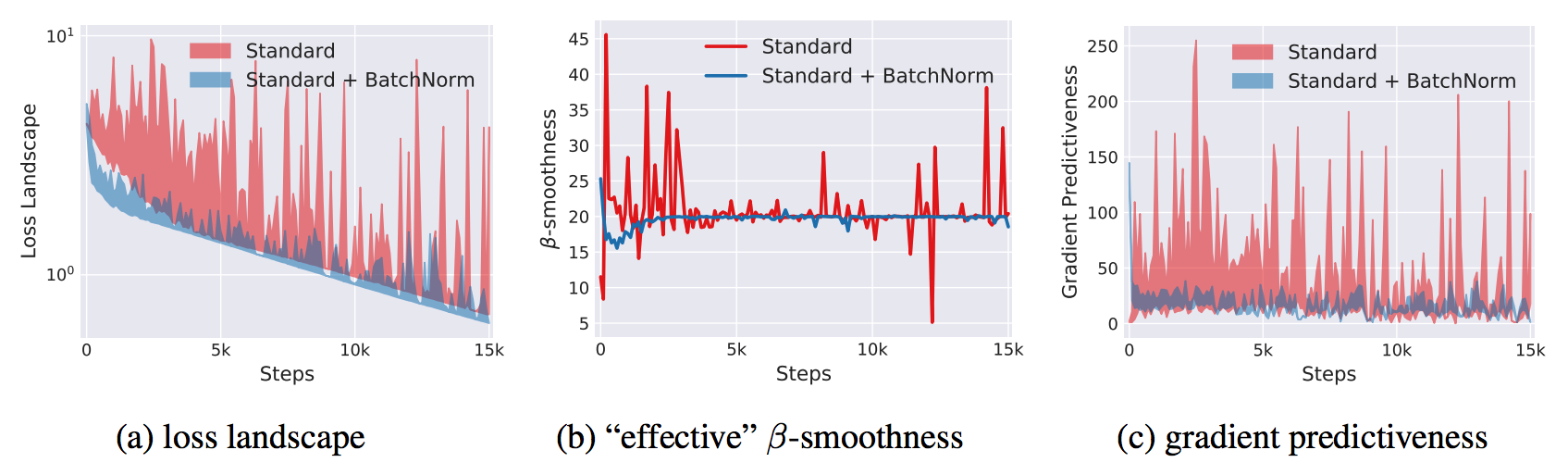
Santurkar and Tsipras et al. argued that the key impact of BN is that it reparametrizes the underlying optimization problem to make its landscape significantly more smooth. With BN,

• The loss landscape is smoother and has less discontinuity (i.e. kinks, sharp minima). The loss changes at a smaller rate and the magnitudes of the gradient is smaller too. In other words, the Lipschitzness of the loss function is improved. (a function f is L-Lipschitz, $ \vert f(x_1) - f(x_2) \vert \leq L \vert \vert x_1 - x_2 \vert \vert $)
• Improved Lipschitzness of the gradients gives us confidence that when we take a larger step in a direction of a computed gradient, this gradient direction remains a fairly accurate estimate of the actual gradient direction after taking that step.
• The gradients are more stable and changes more reliably and predictively. In other words, the loss exhibits a significantly better “effective” $\beta$-smoothness. (a function f is $\beta$-smooth if its gradients are $\beta$-Lipschitz, i.e. $ \vert \vert \nabla f(x_1) - \nabla f(x_2) \vert \leq \beta \vert \vert x_1 - x_2 \vert \vert $)
• Improved Lipschitzness of the gradients gives us confidence that when we take a larger step in a direction of a computed gradient, this gradient direction remains a fairly accurate estimate of the actual gradient direction after taking that step.