Recently, I have been working on the TalkingData AdTracking Fraud Detection Challenge. This is my first experience with CTR prediction, which is similar to NLP and Recommendation Systems in a way that features are very sparse. Field-aware Factorization Models have been dominating the last few CTR prediction competitions on Kaggle so here is my a little write-up for Field-aware Factorization Models and the its origin - Factorization Model.
1. Factorization Machines (FM)
- The most common prediction task is to estimate a function $y: \mathcal{R}^n \rightarrow T$ from a real valued feature vector $\textbf{x} \in \mathcal{R}^n$ to a target domain $T$ ($T = \mathcal{R}$ for regression or $T = \{+, -\}$ for classification)
- Under sparsity, almost all of the elements in $\textbf{x}$ are zero. Huge sparsity appears in many real-world data like recommender systems or text analysis. One reason for huge sparsity is that the underlying problem deals with large categorical variable domains.
- The paper uses the following example of transaction data of a movie review system, with user $u \in U$ rates a movie $i \in I$ at a time $t \in \mathcal{R}$ with a rating $r = \{1, 2, 3, 4, 5\}$
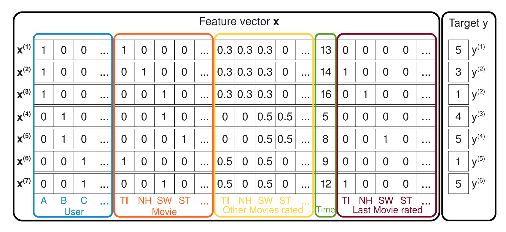
- The above figure shows an example of how feature vectors can be created.
-
$ U $ and $ I $ binary indicators variables for the active user and item, respectively - Implicit indicators of all other movies the users has ever rated, normalized to sum up to 1
- Binary indicators of the last movie rated before the current one
-
1.1 Factorization Machine Model
-
The equation for a factorization machine of degree $d = 2$ \(\hat{y}(\textbf{x}) = w_0 + \sum_{i=1}^n w_i x_i + \sum_{i=1}^n \sum_{j=i+1}^n \langle \textbf{v}_i, \textbf{v}_j \rangle x_i x_j \tag{1}\) where $w_0 \in \mathcal{R} \ \ \textbf{w} \in \mathcal{R}^n \ \ \textbf{V} \in \mathcal{R}^{n \times k}$
- A row $\textbf{v}_i$ describes the i-th variable with k-factors. $k$ is a hyperparameter that defines the dimensionality of the factorization
- The 2-way FM captures all single and pairwise interactions between variables
- $w_0$ is the global bias, $w_i$ models the strength of the i-th variable
- $\hat{w}_{i,j} = \langle \textbf{v}_i, \textbf{v}_j \rangle$ models the interaction between i-th and j-th variable. The FM models the interaction by factorizing it, which is the key point which allows high quality parameter estimates of higher-order interactions under sparsity
-
Expressiveness: For any positive definite matrix $\textbf{W}$, there exists a matrix $\textbf{V}$ such that $W = \textbf{V}\textbf{V}^T$ if $k$ is large enough. Thus, FM can express any interaction matrix $\textbf{W}$ if $k$ is chosen large enough. However, in sparse settings, typically a small $k$ should be chosen because there is not enough data to estimate complex interactions. Restricting $k$ and the expressiveness of FM often lead to better generalization under sparsity.
-
Parameter Estimation Under Sparsity: FM can estimate interactions even in sparse settings well because they break the independence of the interaction parameters by factorizing them. This means that the data for one interaction helps also to estimate the parameters for related interactions.
- Computation: The complexity of straight forward computational of Eq. 1 is in $O(kn^2)$ due to pairwise interactions. With the kernel trick, the model equation can be computed in linear time $O(kn)$
1.2 Loss Function of FM
- Regression: $\hat{y}(\textbf{x})$ can be used directly as the predicator and the loss is MSE
- Binary Classification the sign of $\hat{y}(\textbf{x})$ is used and the loss is the hinge loss or logit loss
- Ranking: the vectorr $\textbf{x}$ are odered by the score of $\hat{y}(\textbf{x})$ and loss is calculated over pairs of vectors with a pairwise classification loss
1.3 Learning Factorization Machines
Since FM has a closed model equation, the model parameters $w_0, \textbf{w}, \textbf{V}$ can be learned efficiently by gradient descent methods for a varity of loss.
\[\frac{\partial }{\partial \theta}\hat{y}(\textbf{x}) = \begin{cases} 1, & \theta = w_0 \\\\ x_i, & \theta = w_i \\\\ x_i \sum_{i=1}^n v_{i,f} x_i - v_{i,f} x_i^2, & \theta = v_{i, f} \end{cases}\]1.4 d-way FM
The 2-way FM can easily be generalized into a d-way FM and it can still be computed in linear time.
2. FM vs SVM
- The model equation of an SVm can be expressed as the dot product between the transformed input $\textbf{x}$ and model parameter $\textbf{w}$, $\hat{y}(\textbf{x}) = \langle \phi(\textbf{x}), \textbf{w} \rangle$, where $\phi$ is a mapping from the feature space $\mathcal{R}^n$ to a more complex space $\mathcal{F}$.
- We can define the kernel as $K(\textbf{x}, \textbf{z}) = \langle \phi(\textbf{x}), \phi(\textbf{z}) \rangle$
2.1 SVM Model
Linear Kernel
- The linear kernel is $K(\textbf{x}, \textbf{z}) = 1 + \langle \textbf{x}, \textbf{z} \rangle$, which translate to the mapping $\theta(\textbf{x}) = [1, x_1, \cdots, x_n]$.
- The model equation of a linear SVM can also be written as $\hat{y}(\textbf{x}) = w_0 + \sum_{i=1}^n w_i x_i$, which is identical to FM with degree $d = 1$
Polynomial Kernel
- The polynomial kernel $K(\textbf{x}, \textbf{z}) = (1 + \langle \textbf{x}, \textbf{z} \rangle)^d$ allow the SVM to model higher interactions between variables.
- For $d = 2$, the polynomial SVMs can be written as \(\hat{y}(\textbf{x}) = w_0 + \sqrt{2}\sum_{i=1}^n w_i x_i + \sum_{i=1}^n w_{i,i}^{(2)} x_i^2 + \sqrt{2}\sum_{i=1}^n \sum_{j=i+1}^n w_{i,j}^{(2)} x_i \tag{1}\)
- The main difference between a polynomial SVM (eq (2)) and the FM with degree $d = 2$ (eq (1)) is the parameterization: all interaction parameters $w_{i,j}$ of SVMs are completely independent. In contrast to the this, interaction parameters of FMs are factorized and $\langle \textbf{v}_i, \textbf{v}_j \rangle$ and $\langle \textbf{v}_i, \textbf{v}_l \rangle$ dependent on each other
2.2 Parameter Estimation Under Sparsity
- For very sparse problems in collaborative filtering settings, linear and polynomial SVMs fail.
- This is primarily due to the fact that all interaction parameters of SVMs are independent. For a reliable estimate of the interaction parameter $w_{i,j}$, there must be enough data points where $x_i \neq 0$ and $x_j \neq 0$. As soon as either $x_i = 0$ or $x_j$, the case $\textbf{x}$ cannot be used for estimating the parameter $w_{i,j}$. If the data is too sprase, SVMs are likely to fail due to too few or even no cases for $(i,j)$
3. Field-aware Factorization Machine (FFM)
- A variant of FMs, field-aware factorization machiens (FFMs), have been outperforming existing models in a number of CTR-prediction competitions (Avazu CTR Prediction and Criteo CTR Prediction)
- The key idea in FFM is field and each feature has several latent vectors, depending on the field of other features.
| Clicked | Publisher (P) | Advertiser (A) | Gender (G) |
|---|---|---|---|
| Yes | ESPN | Nike | Male |
- For the above example, FM will model it as (neglecting the bias terms), \(\hat{y}_{FM} = \langle v_{ESPN}, v_{Nike} \rangle + \langle v_{ESPN}, v_{Male} \rangle + \langle v_{Male}, v_{Nike} \rangle\)
- In FM, eveyr feature has only one latent vector to learn the latent effect with any other features. $v_{ESPN}$ is used to learn the latent effect with Nike $\langle v_{ESPN}, v_{Nike} \rangle$ and Male $\langle v_{ESPN}, v_{Male} \rangle$. However, Nike and Male belong to different fields so the latent efects of (ESPN, Nike) and (ESPN, Male) may be different.
-
In FFM, each feature has several latent vectors. Depending on the field of other features, one of them is used to do the inner product. For the same example, FFM will model it as \(\hat{y}_{FFM} = \langle v_{ESPN,A}, v_{Nike,P} \rangle + \langle v_{ESPN,G}, v_{Male,P} \rangle + \langle v_{Male,G}, v_{Nike,A} \rangle\)
- Neglecting the global bias terms, the model equation of degree $d = 2$ FM is defined as \(\hat{y}(\textbf{x}) = \sum_{i=1}^n \sum_{j=i+1}^n \langle \textbf{v}_i, \textbf{v}_j \rangle x_i x_j \tag{3}\)
- the model equation of degree $d = 2$ FFM is defined as \(\hat{y}(\textbf{x}) = \sum_{i=1}^n \sum_{j=i+1}^n \langle \textbf{v}_i^{(J)}, \textbf{v}_j^{(I)} \rangle x_i x_j \tag{4}\) where $I$ and $J$ are the fields of $i, j$
- If $m$ is the number of fields, the total parameters of FFM is $mnk$ and the total parameter of FM is $nk$
- The time complexity of FFM is $O(kn^2)$ and the time complexity of FM is $O(kn)$