I have been working on some NLP-related Kaggle competitions lately and have came across the Highway Networks in quite a few papers and models. The LSTM-inspired Highway Networks make it easier to train deep networks by adding a small twick to the vanilla feedforward layer. I am reading the paper to get an intuition of how they work.
1. Introduction
- It’s well known that deep networks can represent certain function classes exponentially more efficiently than shallow ones. However, optimization of deep networks is considerably more difficult.
- Srivastava et al. presented a architecture that enables the opmiziation of networks with virtually arbitary depth by a learned gating mechanism for regulating information flow. A network can have paths along which information can flow across several layers without attenuation.
2. Highway Networks
-
For a layer in a plain feedforward network \(\mathbf{y} = H(\mathbf{x}, \mathbf{W}_{H})\) where H is an affine transfor following by a non-linear activation function.
-
For a highway network, we define two non-linear transforms $T(\mathbf{x}, \mathbf{W}_T)$ and $C(\mathbf{x}, \mathbf{W}_C)$ such that \(\mathbf{y} = H(\mathbf{x}, \mathbf{W}_{H}) \cdot T(\mathbf{x}, \mathbf{W}_T) + \mathbf{x} \cdot C(\mathbf{x}, \mathbf{W}_C)\)
-
$T$ is the transform date and $C$ is the carry gate, each respectively express how much of the output is produced by transforming the input and carrying it.
-
For simplicity, we set $C = 1 - T$, giving \(\mathbf{y} = H(\mathbf{x}, \mathbf{W}_{H}) \cdot T(\mathbf{x}, \mathbf{W}_T) + \mathbf{x} \cdot (1-T(\mathbf{x}, \mathbf{W}_C))\)
-
This re-parametrization of the layer transformation is more flexible than the plain feedforward layer. Since \(\mathbf{y} = \begin{cases} \mathbf{x}, & \text{if} \ \ T(\mathbf{x}, \mathbf{W}_C) = 0 \\\\ H(\mathbf{x}, \mathbf{W}_{H}), & \text{if} \ \ T(\mathbf{x}, \mathbf{W}_C) = 1 \end{cases}\) \(\frac{d\mathbf{y}}{d\mathbf{x}} = \begin{cases} \mathbf{I} = 0 \\\\ H'(\mathbf{x}, \mathbf{W}_{H}), & \text{if} \ \ T(\mathbf{x}, \mathbf{W}_C) = 1 \end{cases}\)
-
Depending on the output of the transform gates $(\mathbf{x}, \mathbf{W}_C)$, a highway layer can smoothly vary its behavior between a plain layer and a layer that simply passes its inputs through.
-
For highway layers, we user the tranform gate defined as \(T(\boldsymbol{x}) = \sigma(\boldsymbol{W}_T^T + \boldsymbol{b}_T)\)
-
For training very deep networks, $\boldsymbol{b}_T$ can be initallzed with a negative value such that the network is initially biased towards carrry behavior.
Experiments and Analysis
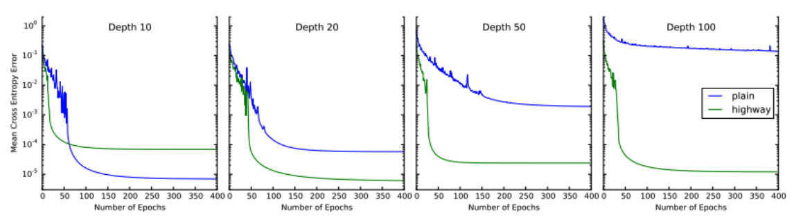
- Networks with depths of 10, 20, 50 and 100 plain or highway layers are trained.
- Optimization: The performance of plain networks degrades significantly as depth increases, while highway networks do not seem to suffer from an increase in depth at all.
-
Performance: The performance of highway networks is similar to Fitnets on CIFAR-10 and MNIST datasets. But highway network is much easier to train since no two-stage training procedure is needed.
-
Analysis: By analzing the biases of the transform gates and the outputs of the block, it was found that the strong negative biases at low depths are not used to shut down the gates, but to make them more selective.