This was an homework problem in STATS315A Applied Modern Statistics: Learning at Stanford and I thought it is worth sharing. It runs a simulation to compare KNN and linear regression in terms of their performance as a classifier, in the presence of an increasing number of noise variables.
Model
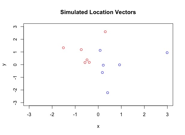
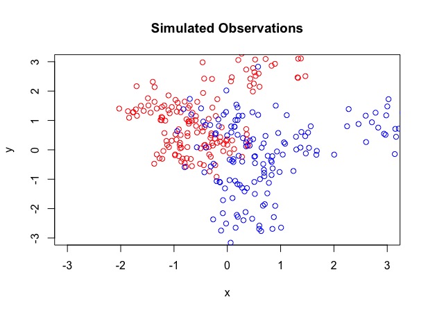
We have a binary response variable $Y$, which takes value ${0,1}$. The feautre variable $X$ is in $\mathcal{R}^{2 + k}$, of which 2 are the true features and the rest $k$ are noise features. The model used to simulate the data is a Gaussian Mixture. First we generate 6 location vectors $m_{k}$ in $\mathcal{R}^{2}$ from a bivariate Gaussian $N[(1,0)^{T}, \boldsymbol{I}]$ with $Y = 1$ and 6 location vectors from $N[(0,1)^{T}, \boldsymbol{I}]$ with $Y = 0$. To simulate $n$ observations from each class, we picked an location vector $m_k$ with a probaility of $1/6$ and then generate one observation from $N[m_k, \boldsymbol{I}/5]$.
Data Simulation
set.seed(1)
library(MASS)
library(mvtnorm)
library(class)
# generate the location vectors with multivariate gaussian
class_0_loc_vec <- mvrnorm(n = 6, c(0,1), diag(2))
class_1_loc_vec <- mvrnorm(n = 6, c(1,0), diag(2))
class_loc_vec <- rbind(class_0_loc_vec, class_1_loc_vec)

# function to generate sample points from the gaussian mixture
sample_points <- function(centroid, N, sigma2) {
  # function to generate a sample point, given a location vector
  simulate_points <- function(centroidNum) {
    return(mvrnorm(n=1, centroid[centroidNum,], sigma2 * diag(2)))
  }
  # randomly choose from the 6 location vectors from class 0
  random_centrod_0 <- sample(1:6, N/2, replace=T)
  X_0 <- sapply(random_centrod_0, simulate_points)
  # randomly choose from the 6 location vectors from class 1
  random_centrod_1 <- sample(7:12, N/2, replace=T)
  X_1 <- sapply(random_centrod_1, simulate_points)
  return(rbind(t(X_0), t(X_1)))
}

# generate a training set of 200 and a test set of 20k, half and half for class 0 and 1
xtrain <- sample_points(class_loc_vec, 300, 0.2)
ytrain <- rbind(matrix(0, 150, 1), matrix(1, 150, 1))
xtest <- sample_points(class_loc_vec, 20000, 0.2)
ytest <- rbind(matrix(0, 10000, 1), matrix(1, 10000, 1))
Bayes Clasifier
Given that we know the underlyign model, we can compute the Bayes Classifier \(\hat{Y}(x) = \text{argmax}_Y(Pr(Y|X=x))\) In our case, we can find the closest location vector to an observation and assign the observation to its class.
# bayes classifier
bayes_classifier <- function(centroid, X, sigma) {
  # due to equal covariance, we only need to find closest centroid and assign it to its class
  findClosestCentroid <- function(index) {
    evaluate_density <- function(ccentroid_index, index) {
      return(dmvnorm(X[index,], centroid[ccentroid_index,], sigma = sigma^2 * diag(2)))
    }
    densities <- sapply(1:12, evaluate_density, index = index)
    return(which.max(densities))
  }
  n <- dim(X)[1]
  assigned_centroids <- sapply(1:n, findClosestCentroid)
  y_pred <- sapply(assigned_centroids, function(x){if (x < 7) return(0) else return(1)})
  return(y_pred)
}
Function to Add Noise
We adds up to $K$ noise features to the training data, drawing each noise observations from the uniform normal distribution $N(0,1)$
# function to add noise
add_noise <- function(data, noise, sigma.noise) {
  noise <- mvrnorm(n = dim(data)[1], rep(0, noise), sigma.noise^2 * diag(noise))
  data_noise <- cbind(data, noise)
  return(data_noise)
}
Function to Evaluate Accuracy and Plot
# function to evaluate knn error with a vector of k
evaluate_knn_vec <- function(xtrain, xtest, ytrain, ytest, k_vec) {
  evaluate_knn <- function(k) {
    knn_pred = knn(train = xtrain, test = xtest, k = k, cl = ytrain)
    return(1-sum(knn_pred == ytest)/length(ytest))
  }
  knn_test_error = sapply(k_vec, evaluate_knn)
  return(knn_test_error)
}
# function to evaluate least squares classifiers test errors
evaluate_ls <- function(xtrain, xtest, ytrain, ytest) {
  xtrain <- cbind(xtrain, matrix(1, dim(xtrain)[1], 1))
  xtest <- cbind(xtest, matrix(1, dim(xtest)[1], 1))
  beta <- solve(t(xtrain) %*% xtrain) %*% t(xtrain) %*% ytrain
  y_pred_numeric <- xtest %*% beta
  y_pred <- sapply(y_pred_numeric, function(x){if (x < 0.5) return(0) else return(1)})
  return(1 - sum(y_pred == ytest)/length(ytest))
}
# function to evaluate bayes classifiers test errors
evaluate_bayes <- function(centroid, X, Y,sigma) {
  y_pred <- bayes_classifier(centroid, X, sigma)
  return(1-sum(y_pred == Y)/length(Y))
}
# function to compute all errors with added noise, color argument is for plotting on the same figure
compute_plot_errors <- function(noise, sigma.noise, color) {
  xtrain <- add_noise(xtrain, noise, sigma.noise)
  xtest <- add_noise(xtest, noise, sigma.noise)
  k <- c(1, 3, 5, 7, 9, 11, 13, 15)
  knn_error <- evaluate_knn_vec(xtrain, xtest, ytrain, ytest, k)
  ls_error <- evaluate_ls(xtrain, xtest, ytrain, ytest)
  if (noise == 1) {
    plot(k, knn_error, type = "b", pch = 16,ylim = c(0, 0.3), col = color, xlab = "k/DoF", ylab = "Test Error")
  }
  else {
    points(k, knn_error, type = "b", pch = 16,ylim = c(0, 0.3), col = color)
  }
  points(3+noise, ls_error, pch = 18)
  abline(h=bayes_error, col="brown")
}
Simulate Performance for $K = 1 \cdots 10$
colors = palette(rainbow(10))
for (noise in 1:10) {
  compute_plot_errors(noise, 1, colors[noise])
}
x <- 1:10
legend_names <- c(paste("Noise", x), "Least Squares","Bayes Error")
legend("bottom",legend_names,fill=c(colors, "black", "brown"),ncol=4, cex = 0.9)
Results
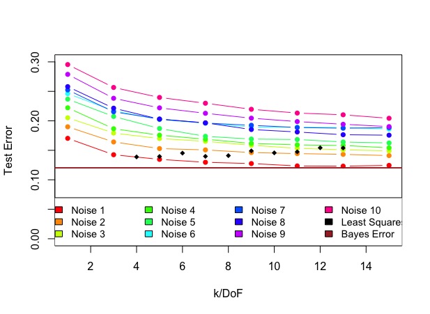
Overall, the test error of KNN decreases as $k$ increases, no matter how many noise parameters there are The test error of KNN generally increases significantly as the number of noise parameters increases, while the test error of least squares stays at about the same level. This shows that the KNN is more susceptible to high noise due to its flexiblity. The least squares is more rigid and is less affected by the noise. KNN overperforms the least squares when the noise-to-signal ratio is low and underperforms the least squares when the noise-to-signal ratio is high.